Clustering

Broad set of techniques for finding subgroups.
Observations within groups are quite similar to each other and observations in different groups quite different from each other.

Clustering methods

Partitioning: k-means clustering
Agglomerative/divisive: hierarchical clustering
Model-based: mixture models

K-means clustering

Simple approach to partitioning a data set into K distinct, non-overlapping clusters.
K is specified beforehand.

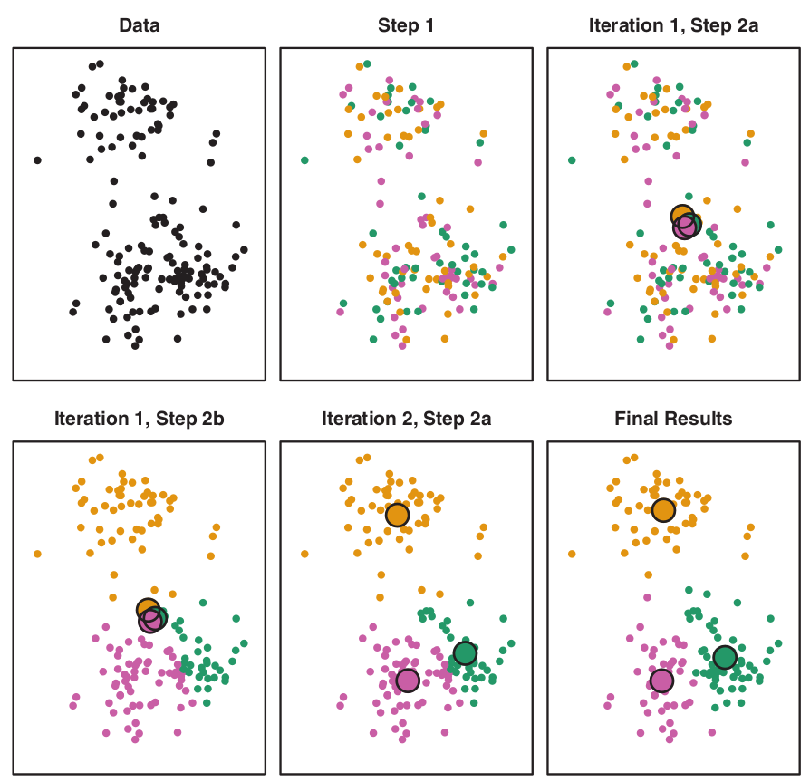
K-means algorithm

\(K\) – number of clusters.

The process:

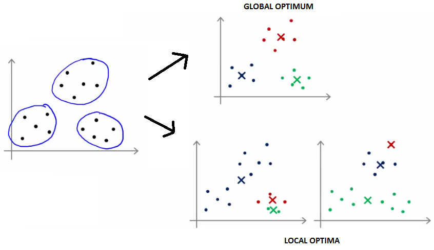
Randomly assign each observation to groups 1 to K;
For each of K clusters, derive its centroid (midpoint);
Reassign each observation into a cluster whose centroid is the closest;
Iterate until stability in cluster assignments is reached (local vs global optima).

Some properties of K-means partitioning

Standard algorithm for k-means clustering is using Euclidean distance (distances are calculated using Pythagorean theorem).
Different local optima (stability) can be reached.

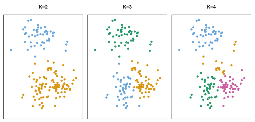
Number of clusters K must be specified in advance
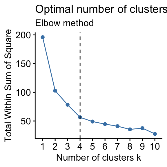
How to determine optimal number of clusters?
- Elbow method,
- Silhouette method

PCA

library(dplyr)
library(tidyr)
library(ggplot2)

# Data preparation ----
# Read data on dart points
dartpoints <- read.csv("data/dartpoints.csv")

# Filter to two types of dart points, select numeric columns
# and remove rows with missing values
dp <- dartpoints |> 
  filter(Name %in% c("Darl", "Pedernales")) |> 
  select(Name, where(is.numeric)) |> 
  drop_na()

head(dp, 4)

  Name Length Width Thickness B.Width J.Width H.Length Weight
1 Darl   42.8  15.8       5.8    11.3    10.6     11.6    3.6
2 Darl   37.5  16.3       6.1    12.1    11.3      8.2    3.6
3 Darl   40.3  16.1       6.3    13.5    11.7      8.3    4.0
4 Darl   30.6  17.1       4.0    12.6    11.2      8.9    2.3

tail(dp, 4)

         Name Length Width Thickness B.Width J.Width H.Length Weight
40 Pedernales   56.2  22.6       8.5    13.5    18.4     18.3    9.4
41 Pedernales   47.1  20.9       7.5    13.6    18.2     18.5    6.7
42 Pedernales   64.1  27.2      10.2    13.2    17.0     15.5   15.1
43 Pedernales   65.0  31.6      10.1    10.9    17.7     23.0    4.6

Scatterplot

# Scatter plot of Length vs Weight colored by Name
dp |> 
  ggplot(aes(x = Length, y = Weight, color = Name)) +
  geom_point() +
  theme_minimal()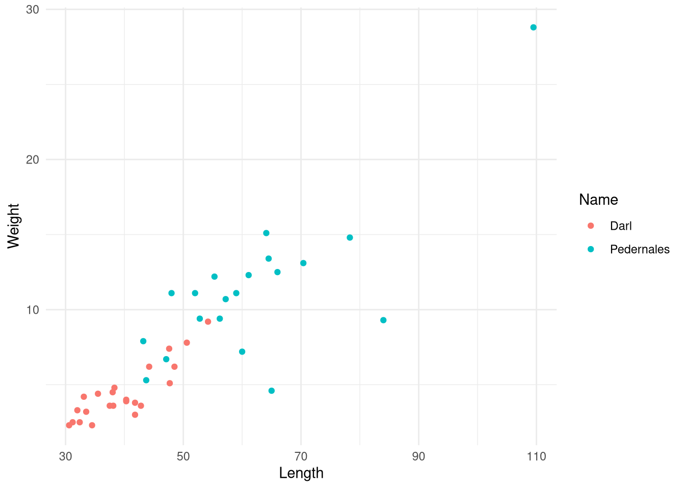

Reduce dimensions using PCA

# PCA analysis ----
# Prepare data matrix for PCA
dp_matrix <- dp |> 
  select(where(is.numeric)) |> 
  as.matrix()

rownames(dp_matrix) <- dp |> pull(Name) # add rownames

# Scale data to remove effects of different units and magnitudes
scaled <- scale(dp_matrix, center = TRUE, scale = TRUE)

# PCA analysis
pca <- prcomp(scaled)
# alternatively prcomp(dp_matrix, center = TRUE, scale. = TRUE))

# Summary of PCA results
summary(pca)

Importance of components:
                          PC1    PC2     PC3    PC4     PC5     PC6     PC7
Standard deviation     2.1378 1.0104 0.80296 0.5898 0.46825 0.34354 0.28090
Proportion of Variance 0.6529 0.1459 0.09211 0.0497 0.03132 0.01686 0.01127
Cumulative Proportion  0.6529 0.7987 0.89085 0.9405 0.97187 0.98873 1.00000

Biplot

# Biplot with color mapped to Name
biplot(pca)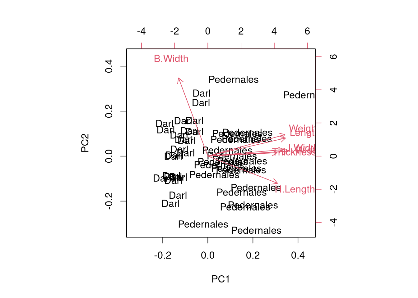

ggplot2 biplot

# ggplot2 'biplot' visualization
pca_scores <- as.data.frame(pca$x)

# Add variation to biplot axis labels
var_explained <- round(100 * (pca$sdev^2) / sum(pca$sdev^2), 1)

pca_scores |> 
  ggplot() +
  aes(x = PC1, y = PC2, color = dp$Name) +
  geom_point(size = 3) +
  theme_minimal() +
  coord_fixed() +
  labs(title = "PCA Biplot of Dart Points",
       x = paste0("PC1 (", var_explained[1], "%)"),
       y = paste0("PC2 (", var_explained[2], "%)"),
       color = "Dart point type")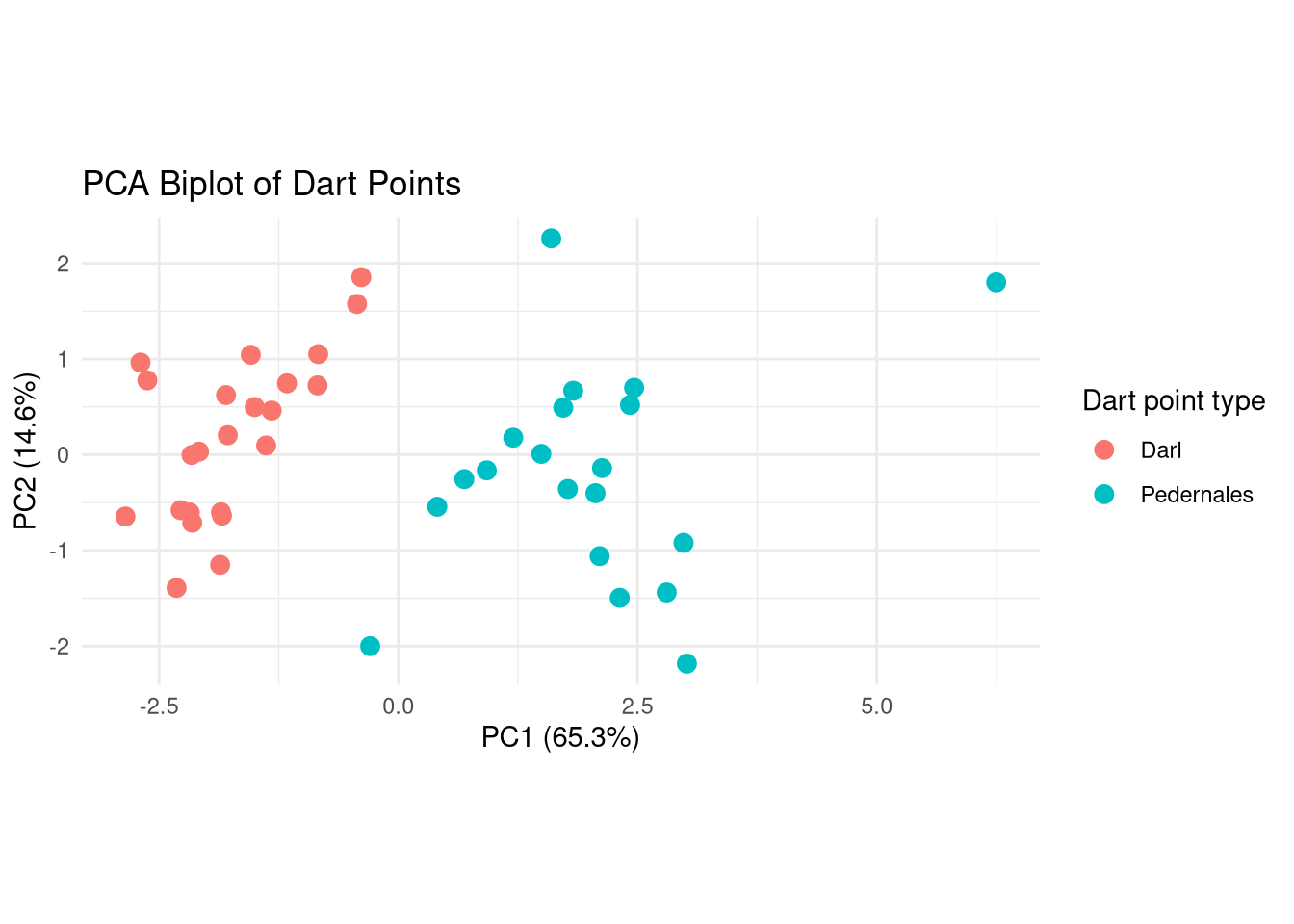

How many clusters?

# K-means clustering ----
# Set seed (random number generator) for reproducibility
set.seed(42)

# Elbow method to determine optimal number of clusters
# factoextra::fviz_nbclust(pca_scores[, 1:2], kmeans, method = "wss")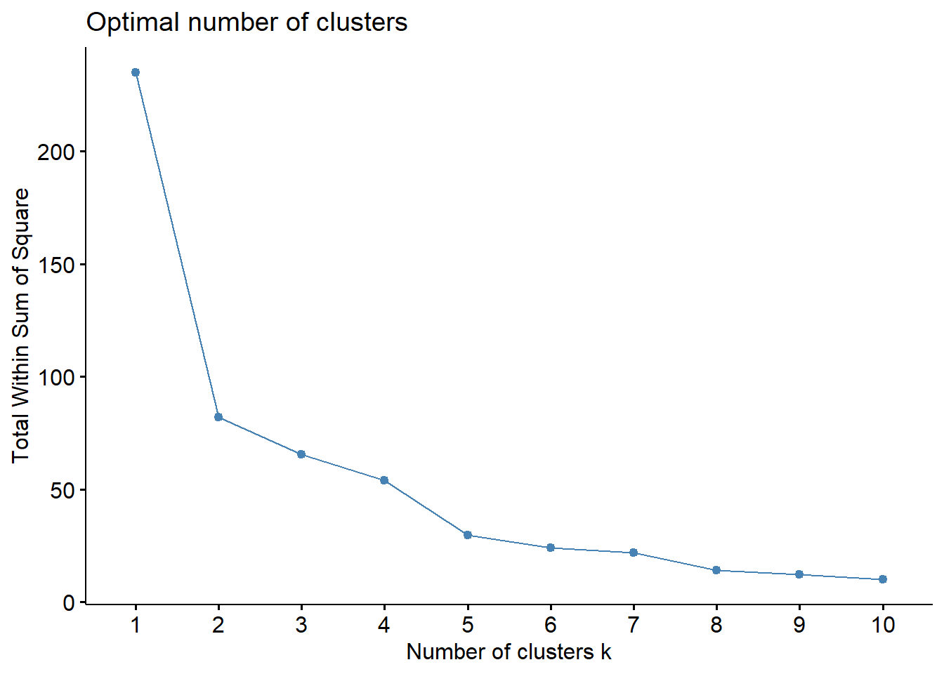

K-means

# Caculate K-means
kmeans_result <- kmeans(pca_scores, centers = 2, nstart = 25)

kmeans_result

K-means clustering with 2 clusters of sizes 19, 24

Cluster means:
        PC1         PC2        PC3         PC4         PC5         PC6
1  2.114733 -0.12266480 -0.1703675  0.02350401 -0.04361522  0.03322302
2 -1.674164  0.09710964  0.1348743 -0.01860734  0.03452871 -0.02630156
          PC7
1  0.01907226
2 -0.01509887

Clustering vector:
         Darl        Darl.1        Darl.2        Darl.3        Darl.4 
            2             2             2             2             2 
       Darl.5        Darl.6        Darl.7        Darl.8        Darl.9 
            2             2             2             2             2 
      Darl.10       Darl.11       Darl.12       Darl.13       Darl.14 
            2             2             2             2             2 
      Darl.15       Darl.16       Darl.17       Darl.18       Darl.19 
            2             2             2             2             2 
      Darl.20       Darl.21       Darl.22    Pedernales  Pedernales.1 
            2             2             2             1             1 
 Pedernales.2  Pedernales.3  Pedernales.4  Pedernales.5  Pedernales.6 
            1             1             1             1             2 
 Pedernales.7  Pedernales.8  Pedernales.9 Pedernales.10 Pedernales.11 
            1             1             1             1             1 
Pedernales.12 Pedernales.13 Pedernales.14 Pedernales.15 Pedernales.16 
            1             1             1             1             1 
Pedernales.17 Pedernales.18 Pedernales.19 
            1             1             1 

Within cluster sum of squares by cluster:
[1] 88.53841 51.59016
 (between_SS / total_SS =  52.3 %)

Available components:

[1] "cluster"      "centers"      "totss"        "withinss"     "tot.withinss"
[6] "betweenss"    "size"         "iter"         "ifault"

Plot

# Plot
pca_scores |> 
  ggplot() +
  aes(x = PC1, y = PC2, color = factor(kmeans_result$cluster)) +
  geom_point(size = 3) +
  theme_minimal() +
  labs(title = "K-means Clustering on PCA Results",
       x = "PC 1",
       y = "PC 2",
       color = "Cluster")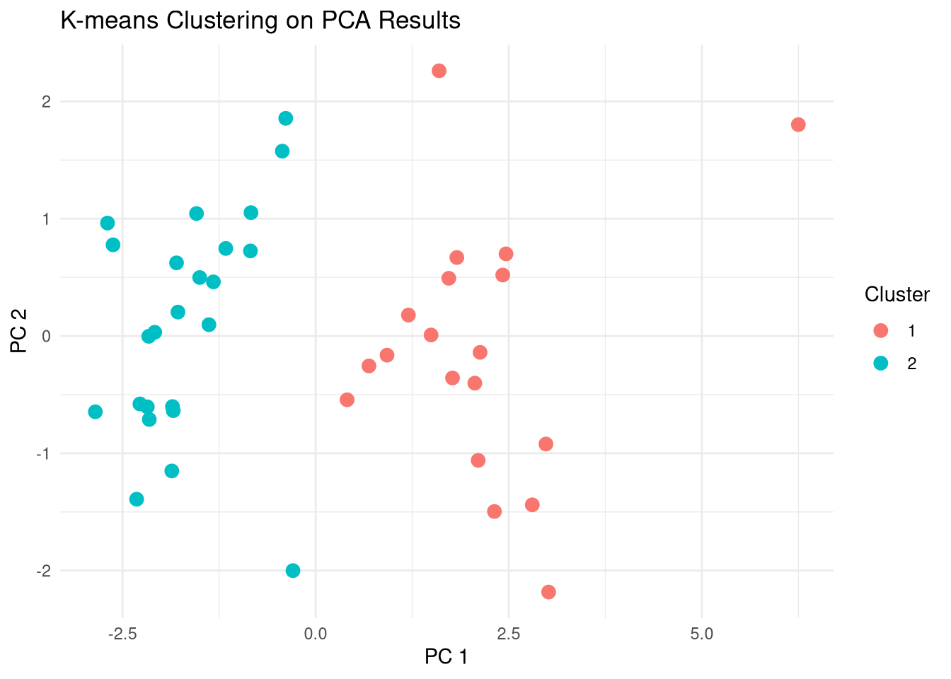

Compare clusters with Names

# Table of clusters vs original names
table(kmeans_result$cluster, dp$Name)

   
    Darl Pedernales
  1    0         19
  2   23          1

# Compare clusters to original names, i.e., dart point types
pca_scores |> 
  ggplot() +
  aes(
    x = PC1, y = PC2, 
    color = dp$Name, 
    shape = factor(kmeans_result$cluster)
  ) +
  geom_point(size = 3) +
  theme_minimal() +
  labs(title = "K-means Clustering on PCA Results",
       x = "PC 1",
       y = "PC 2",
       color = "Type of dartpoint",
       shape = "Cluster")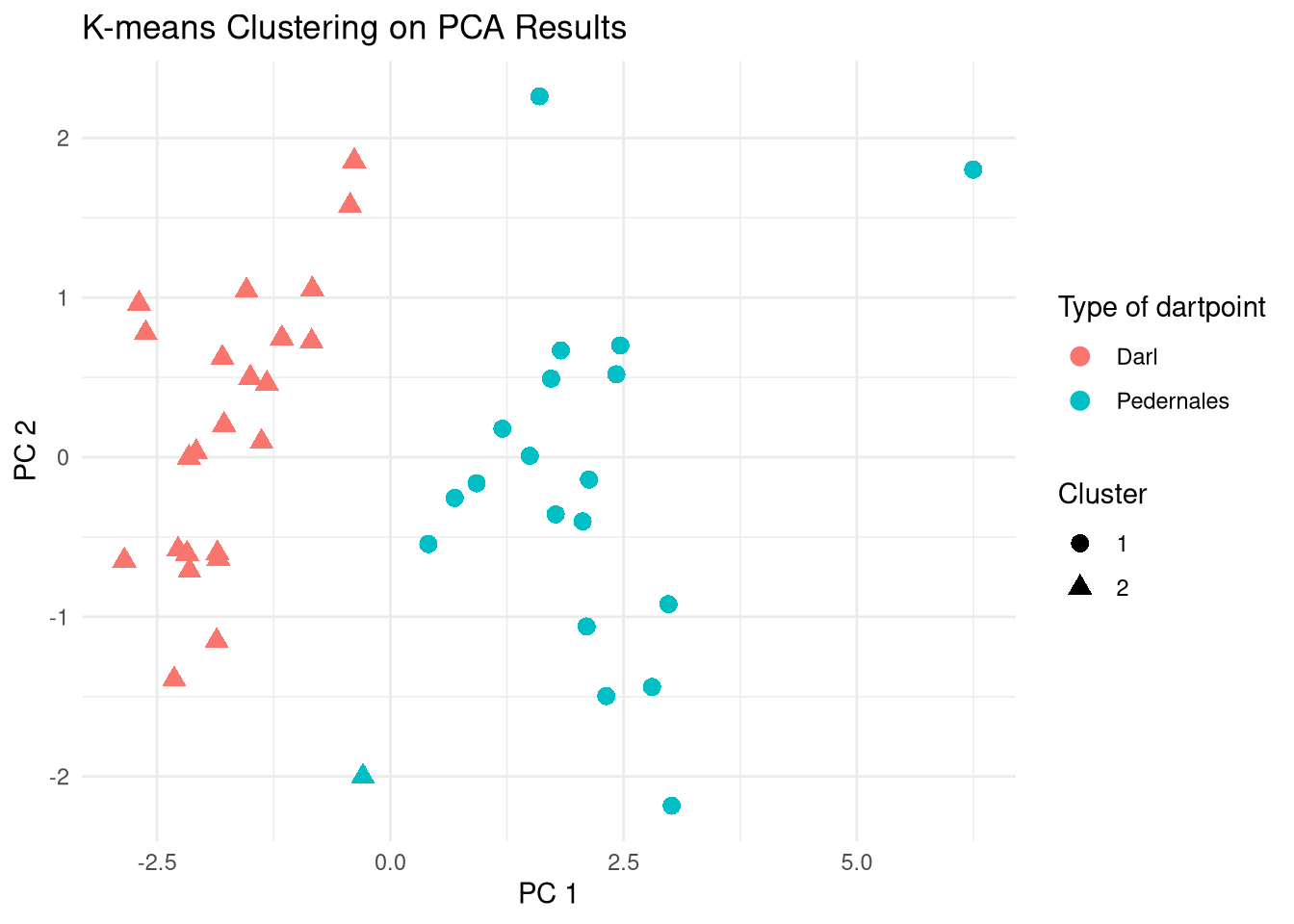

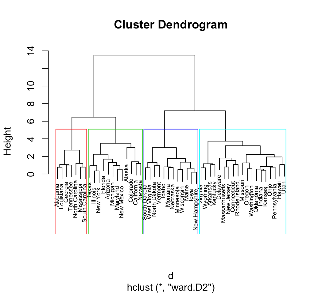
Hierarchical clustering

The number of clusters is not specified beforehand.
Output is a dendrogram – a hierarchical structure visualizing the cluster growth.
Starts with a distance matrix.

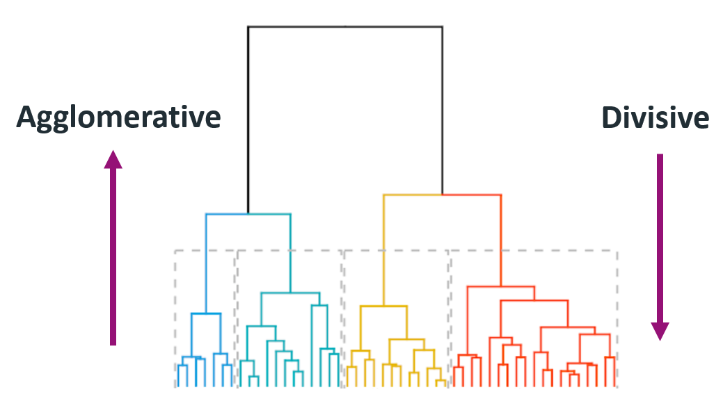
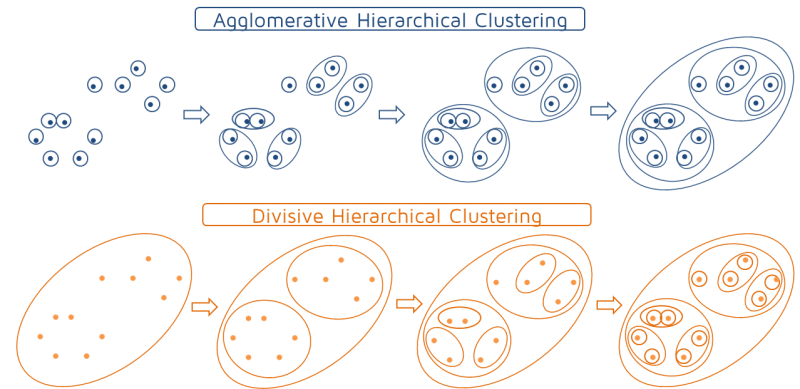
Agglomerative

Builds the hierarchy of clusters from bottom-up until a single cluster is reached.

Put each object in its own cluster;
Join the clusters that are the closest;
Iterate until a single cluster encompassing all objects is reached.

Divisive

Divides a single large cluster into individual objects (top-down).

Put all objects into a single cluster;
Divide the cluster into subclusters at a similar distance;
Iterate util all objects are in their own clusters.

Hierarchical clustering algorithms

Distance matrix

pca_scores[1:5, 1:5]

             PC1         PC2       PC3        PC4         PC5
Darl   -1.861665 -1.15057628 0.5968967 -0.3025608  0.56428007
Darl.1 -2.178930 -0.60404605 0.5255111 -0.7277931 -0.03876516
Darl.2 -2.082508  0.03183789 0.3072156 -0.6342330  0.07207282
Darl.3 -2.851549 -0.64616709 0.8645401  0.3607771 -0.24094772
Darl.4 -2.274738 -0.57920790 0.8686159  0.5521698  0.19617583

# Hierarchical clustering ----

# Calculate distance matrix
dist_matrix <- dist(pca_scores)

as.matrix(dist_matrix)[1:5, 1:5]

           Darl    Darl.1    Darl.2    Darl.3    Darl.4
Darl   0.000000 1.0151059 1.3907752 1.6191148 1.2428550
Darl.1 1.015106 0.0000000 0.6980987 1.3570655 1.4128283
Darl.2 1.390775 0.6980987 0.0000000 1.5855669 1.5079124
Darl.3 1.619115 1.3570655 1.5855669 0.0000000 0.8904547
Darl.4 1.242855 1.4128283 1.5079124 0.8904547 0.0000000

Dendrogram

# Hierarchical clustering using complete linkage
hc <- hclust(dist_matrix, method = "ward.D2")

# Plot dendrogram
plot(hc, labels = dp$Name, main = "Hierarchical Clustering Dendrogram")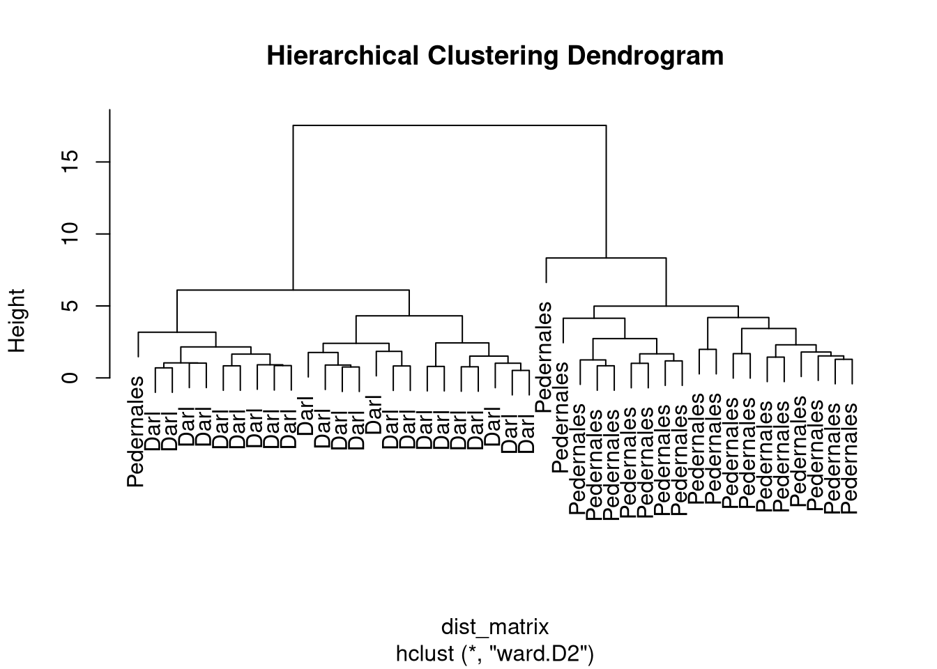

Clusters

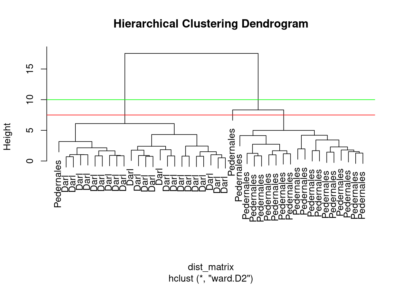
Different options where to cut the dendrogram…
function cutree(x, k, h)
specify k – number of clusters or
h – height where to cut the dendrogram

Cluster assignments

# Cut tree into 2 clusters
hc_clusters <- cutree(hc, k = 2)
unname(hc_clusters)

 [1] 1 1 1 1 1 1 1 1 1 1 1 1 1 1 1 1 1 1 1 1 1 1 1 2 2 2 2 2 2 1 2 2 2 2 2 2 2 2
[39] 2 2 2 2 2

table(hc_clusters, dp$Name)

           
hc_clusters Darl Pedernales
          1   23          1
          2    0         19

Sidenote: Cluster linkage methods

Complete (maximum) linkage

Largest distance between clusters.
method = "complete"

Single (minimum) linkage

Smallest distance between clusters.
method = "single"

Mean (average) linkage

Mean distance between clusters.
method = "average"

Wards method

Minimizes total within cluster variance.
method = "ward.D2"

Clustering methods comparison

K-means partitioning

Pre-specified number of clusters.
Clusters may vary (different local optima).
Best when groups in data are (hyper)spheres.

Hierarchical clustering

Variable cluster numbers.
Clusters are stable.
Any shape of data distribution.