Correspondence analysis

Introduction

In this course, you will learn how to:

do quick correspondence analysis in R
transform your data from long format to wide format
replace NAs with 0
create “tibble” type of tables from vectors
visualize the results of the correspondence analysis in ggplot()

Correspondence analysis (CA) - what is it?

one of the multivariate statistical methods
helps you to explore similarities in your data

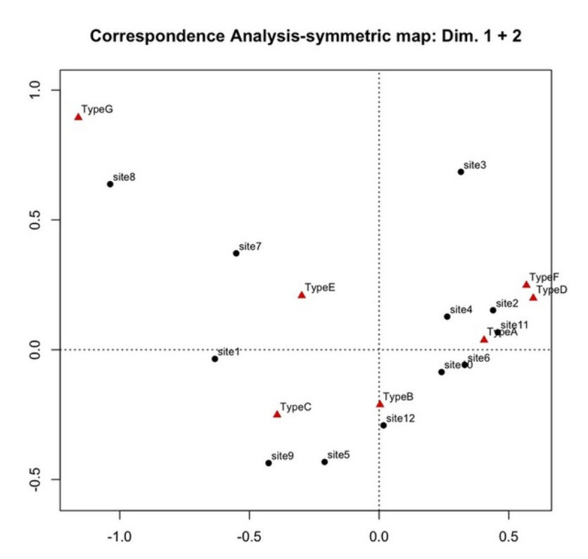
image from: https://cainarchaeology.weebly.com/

the above example shows how the biplot can be used to identify the similarities between different archaeological sites, based on the proportion of different ceramic types found there
note that there are two groups of data: archaeological sites and ceramic types
“similarities are based on proportion…” means that we have counts of ceramic types for each site

Correspondence analysis (CA) - what do I need?

data in the form of a contingency table with the counts of two or more categorical variables
two groups of data: one group in the rows, second in the columns
examples: graves in the rows and counts of their artefacts in the columns, sites and counts of ceramic types, archaeological layers and counts of the chipped stone industry,…
“presence / absence” variables are also suitable but their values have to be replaced by 1 and 0
NAs have to be replaced by 0

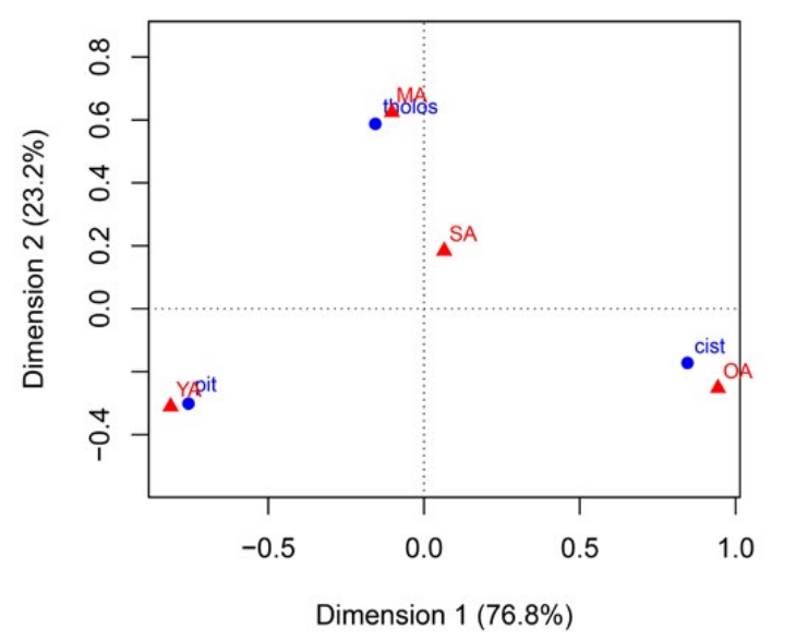
Contingency table

an example of a contingency table:

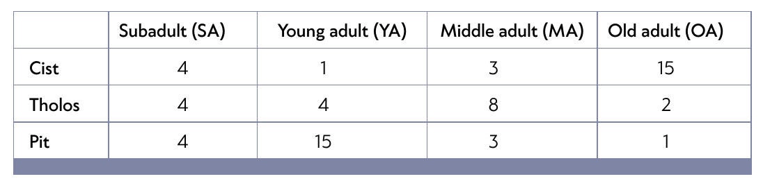
image from: Nikita 2020: INTRODUCTION TO STATISTICS USING R (for archaeologists)

and the biplot showing the result of the CA

Doing CA on artificial archaeological data

Prerequisites

Packages:

here, dplyr, tidyr, ca,tibble, ggplot2

Data:

database “eneol_bronze_burials.csv”

Start:

open your R Project, create a new script file
load packages here, dplyr, tidyr, ggplot2
install and load packages ca and tibble
import the data “eneol_bronze_burials.csv” into R
observe data - what is in rows? what are the variables?

CA - start

install new packages

install.packages("ca")
install.packages("tibble")

load the packages

library(here)
library(dplyr)
library(tidyr)
library(tibble)
library(ggplot2)
library(ca)

import the data

df_graves <- read.csv(here("lect/w04/data/burials.csv"))

observe the data:

df_graves |> 
  arrange(grave_number) |> head(8)

  grave_number dating    sex artefact_type artefact_count artefact_material
1          900 en.zvo   male        beaker              3          ceramics
2          900 en.zvo   male     dartpoint              5           lithics
3          900 en.zvo   male    wristguard              1           lithics
4          900 en.zvo   male        dagger              1            copper
5          900 en.zvo   male           axe              1            copper
6          900 en.zvo   male          bowl              1          ceramics
7          901 en.zvo female        beaker              1          ceramics
8          901 en.zvo female     dartpoint              2           lithics

str(df_graves)

'data.frame':   230 obs. of  6 variables:
 $ grave_number     : int  900 901 902 903 904 905 906 907 908 909 ...
 $ dating           : chr  "en.zvo" "en.zvo" "en.zvo" "en.zvo" ...
 $ sex              : chr  "male" "female" "male" "female" ...
 $ artefact_type    : chr  "beaker" "beaker" "beaker" "beaker" ...
 $ artefact_count   : int  3 1 1 1 1 1 1 2 1 1 ...
 $ artefact_material: chr  "ceramics" "ceramics" "ceramics" "ceramics" ...

Research questions

are there differences between artefacts in different dating periods?
are there differences between the sexes?
are there any similar groups of graves?

to answer the question, we will use correspondence analysis to observe similarities between graves (first group of data) based on similarities in proportion of their artefacts (second group of data)

keep in mind that this database is artificial and for teaching purposes only. Although it might, to some extent, resemble real archaeological data, some aspect were purposely modified to better illustrate the logic of the correspondence analysis

Tidying data

we see that all artefacts are stored in the variable “artefact_type” and their count in “artefact_count”
this table is a type of “long table”, which we were discussing in the last lecture
to do a correspondence analysis, we need to transform this table into so called “wide table”, where one observation will be one grave, and each type of artefact will be one variable
in other words, we need to have a table where:
- one group of data is in rows - in this case graves
- second group of data is in columns - in this case the counts of artefact types

widening data with `tidyr::pivot_wider()`

remember the function pivot_longer() from the tidyr package? Now we will use its reverse sister pivot_wider()
syntax within the pipeline:
df |> pivot_wider(names_from = , values_from = )
names_from - defines the column from which the new variables will be created (e.i. the values in this column will become variables)
values_from - defines from which column the count values will be taken

df_graves_wide <- df_graves |> 
   select(-artefact_material) |> 
   pivot_wider(
    names_from = artefact_type,
    values_from = artefact_count
  )

note that we have removed the variable “artefact_material”

head(df_graves_wide)

# A tibble: 6 × 15
  grave_number dating sex   beaker dartpoint wristguard dagger   axe  bowl  beam
         <int> <chr>  <chr>  <int>     <int>      <int>  <int> <int> <int> <int>
1          900 en.zvo male       3         5          1      1     1     1    NA
2          901 en.zvo fema…      1         2          1     NA    NA     1     2
3          902 en.zvo male       1         2          1     NA    NA     1    NA
4          903 en.zvo fema…      1         2          1     NA    NA     1     2
5          904 en.zvo male       1         2          1     NA    NA     1    NA
6          905 en.zvo fema…      1         2          1     NA    NA     1     3
# ℹ 5 more variables: beam_amber <int>, koflik <int>, bracelet_bronze <int>,
#   needle <int>, spear <int>

Dealing with NAs

now we have to deal with the NAs and turn them into 0
we will use function dplyr::mutate() because we want to change specific values based on specific conditions

df_graves_wide <- df_graves_wide |> 
  mutate(
    across(beaker:spear, ~ replace_na(.x, 0))
  )

head(df_graves_wide)

# A tibble: 6 × 15
  grave_number dating sex   beaker dartpoint wristguard dagger   axe  bowl  beam
         <int> <chr>  <chr>  <int>     <int>      <int>  <int> <int> <int> <int>
1          900 en.zvo male       3         5          1      1     1     1     0
2          901 en.zvo fema…      1         2          1      0     0     1     2
3          902 en.zvo male       1         2          1      0     0     1     0
4          903 en.zvo fema…      1         2          1      0     0     1     2
5          904 en.zvo male       1         2          1      0     0     1     0
6          905 en.zvo fema…      1         2          1      0     0     1     3
# ℹ 5 more variables: beam_amber <int>, koflik <int>, bracelet_bronze <int>,
#   needle <int>, spear <int>

Calculating CA with the function `ca()`

we can conduct the correspondence analysis with the function ca::ca()
NOTE that the CA can be done only on columns with integer data
to proceed, we first need to select the columns with artefact counts, and then run the ca() function
we will incorporate the ca() into the pipe
in this stage it is usefull to use colnames() function to see the column names
in order to CA to work, the sum of each row and column must be greater than zero

colnames(df_graves_wide)

 [1] "grave_number"    "dating"          "sex"             "beaker"         
 [5] "dartpoint"       "wristguard"      "dagger"          "axe"            
 [9] "bowl"            "beam"            "beam_amber"      "koflik"         
[13] "bracelet_bronze" "needle"          "spear"

now we will define which columns to keep for analysis, incorporate the ca() function into the pipe and store the result as “ca_result”

ca_result <- df_graves_wide |> 
  select(beaker:spear) |> 
  ca()

visualising CA result with `plot()`

to quickly visualize the result, we will use the R base function plot() and create the so called biplot:

plot(ca_result)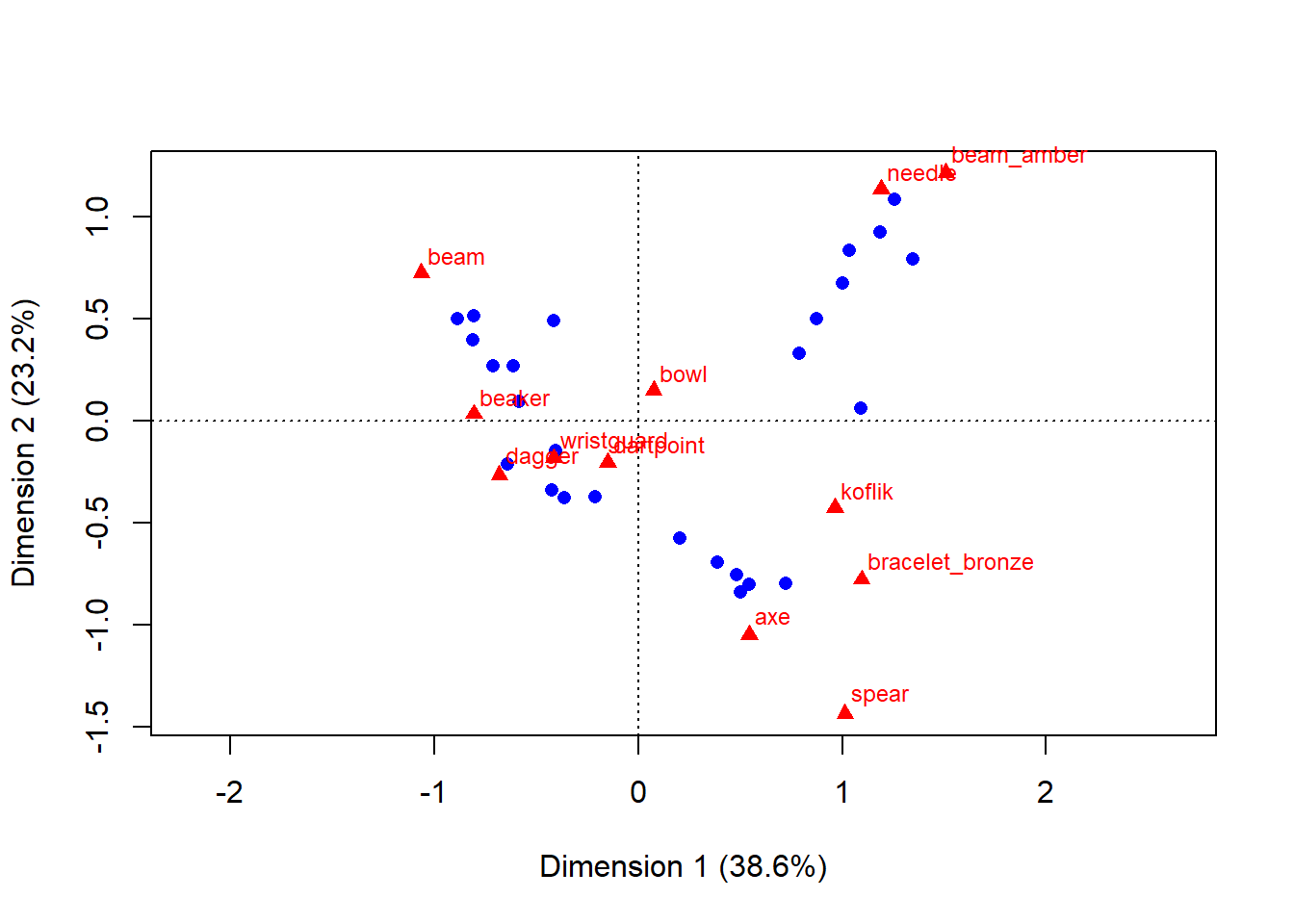

this biplot is basicaly a scatterplot
first group of data - graves - are represented as blue dots, second group - artefacts - are represented as red triangles
each grave and each artefact has it’s own coordinates
the closer the graves or artefacts are to each other, the more similar they are

Observing the results structure

at this stage, we cannot use our beloved ggplot2() function because it works only with dataframes or tables, and the result of the CA is not a dataframe but a list:

str(ca_result)

List of 16
 $ sv        : num [1:11] 0.715 0.555 0.426 0.302 0.28 ...
 $ nd        : logi NA
 $ rownames  : NULL
 $ rowmass   : num [1:50] 0.0345 0.023 0.0144 0.0201 0.0144 ...
 $ rowdist   : num [1:50] 1.04 0.795 0.811 0.811 0.811 ...
 $ rowinertia: num [1:50] 0.03727 0.01451 0.00944 0.01322 0.00944 ...
 $ rowcoord  : num [1:50, 1:11] -0.594 -0.582 -0.565 -0.997 -0.565 ...
  ..- attr(*, "dimnames")=List of 2
  .. ..$ : NULL
  .. ..$ : chr [1:11] "Dim1" "Dim2" "Dim3" "Dim4" ...
 $ rowsup    : logi(0) 
 $ colnames  : chr [1:12] "beaker" "dartpoint" "wristguard" "dagger" ...
 $ colmass   : num [1:12] 0.0948 0.2989 0.1063 0.0115 0.0603 ...
 $ coldist   : num [1:12] 1.03 0.405 0.712 2.42 1.336 ...
 $ colinertia: num [1:12] 0.1006 0.0491 0.0539 0.0673 0.1077 ...
 $ colcoord  : num [1:12, 1:11] -1.127 -0.211 -0.578 -0.954 0.761 ...
  ..- attr(*, "dimnames")=List of 2
  .. ..$ : chr [1:12] "beaker" "dartpoint" "wristguard" "dagger" ...
  .. ..$ : chr [1:11] "Dim1" "Dim2" "Dim3" "Dim4" ...
 $ colsup    : logi(0) 
 $ N         : int [1:50, 1:12] 3 1 1 1 1 1 1 2 1 1 ...
 $ call      : language ca.matrix(obj = as.matrix(obj))
 - attr(*, "class")= chr "ca"

you can see that this is not a dataframe, but a so called “list” with much complicated structure

Observing the results structure 2

And it looks like this:

ca_result


 Principal inertias (eigenvalues):
           1        2        3        4        5        6        7       
Value      0.511633 0.307624 0.181845 0.091006 0.078339 0.059623 0.033804
Percentage 38.58%   23.2%    13.71%   6.86%    5.91%    4.5%     2.55%   
           8        9        10       11      
Value      0.027614 0.022635 0.010099 0.001813
Percentage 2.08%    1.71%    0.76%    0.14%   


 Rows:
             [,1]      [,2]      [,3]      [,4]      [,5]      [,6]      [,7]
Mass     0.034483  0.022989  0.014368  0.020115  0.014368  0.022989  0.008621
ChiDist  1.039607  0.794512  0.810642  0.810643  0.810642  1.022514  1.260380
Inertia  0.037268  0.014511  0.009442  0.013218  0.009442  0.024035  0.013694
Dim. 1  -0.594280 -0.582023 -0.565171 -0.997440 -0.565171 -1.132524 -0.892933
Dim. 2  -0.618500  0.882143 -0.269234  0.480842 -0.269234  0.715240 -0.386827
             [,8]      [,9]     [,10]     [,11]     [,12]     [,13]     [,14]
Mass     0.031609  0.017241  0.014368  0.025862  0.014368  0.008621  0.020115
ChiDist  1.020069  0.653439  0.810642  1.214695  0.810642  1.260380  0.810643
Inertia  0.032891  0.007362  0.009442  0.038159  0.009442  0.013694  0.013218
Dim. 1  -0.505019 -0.817328 -0.565171 -1.237589 -0.565171 -0.892933 -0.997440
Dim. 2  -0.684581  0.168310 -0.269234  0.897550 -0.269234 -0.386827  0.480842
            [,15]     [,16]     [,17]     [,18]     [,19]     [,20]     [,21]
Mass     0.031609  0.057471  0.022989  0.022989  0.008621  0.014368  0.022989
ChiDist  1.020069  1.164693  1.022514  1.022514  1.260380  0.810642  0.805052
Inertia  0.032891  0.077960  0.024035  0.024035  0.013694  0.009442  0.014899
Dim. 1  -0.505019 -1.124728 -1.132524 -1.132524 -0.892933 -0.565171 -0.854313
Dim. 2  -0.684581  0.926668  0.715240  0.715240 -0.386827 -0.269234  0.481463
            [,22]     [,23]     [,24]     [,25]     [,26]     [,27]     [,28]
Mass     0.014368  0.022989  0.014368  0.008621  0.020115  0.008621  0.045977
ChiDist  0.810642  1.022514  0.810642  1.260380  0.810643  1.260380  1.528425
Inertia  0.009442  0.024035  0.009442  0.013694  0.013218  0.013694  0.107406
Dim. 1  -0.565171 -1.132524 -0.565171 -0.892933 -0.997440 -0.892933  1.013292
Dim. 2  -0.269234  0.715240 -0.269234 -0.386827  0.480842 -0.386827 -1.436801
           [,29]     [,30]     [,31]    [,32]     [,33]    [,34]     [,35]
Mass    0.020115  0.031609  0.002874 0.014368  0.017241 0.017241  0.043103
ChiDist 1.720234  1.029241  1.531716 1.286873  0.814505 1.567031  1.127401
Inertia 0.059524  0.033485  0.006742 0.023794  0.011438 0.042338  0.054786
Dim. 1  1.754818  0.539908 -0.294629 1.401986  0.282946 1.659640  0.762122
Dim. 2  1.958447 -1.253150 -0.671498 1.213833 -1.042592 1.669647 -1.452072
           [,36]     [,37]     [,38]    [,39]    [,40]    [,41]    [,42]
Mass    0.017241  0.002874  0.034483 0.022989 0.028736 0.020115 0.025862
ChiDist 1.567031  1.531716  0.999467 1.748814 1.140247 2.130126 0.990176
Inertia 0.042338  0.006742  0.034446 0.070307 0.037361 0.091270 0.025356
Dim. 1  1.659640 -0.294629  0.673294 1.880786 1.224527 1.524143 1.102153
Dim. 2  1.669647 -0.671498 -1.359819 1.429176 0.902438 0.106477 0.592570
            [,43]     [,44]    [,45]     [,46]     [,47]     [,48]    [,49]
Mass     0.002874  0.017241 0.020115  0.037356  0.002874  0.017241 0.014368
ChiDist  1.531716  0.814505 1.426285  1.092480  1.531716  0.814505 1.286873
Inertia  0.006742  0.011438 0.040920  0.044585  0.006742  0.011438 0.023794
Dim. 1  -0.294629  0.282946 1.443630  0.703363 -0.294629  0.282946 1.401986
Dim. 2  -0.671498 -1.042592 1.500527 -1.517977 -0.671498 -1.042592 1.213833
            [,50]
Mass     0.002874
ChiDist  1.531716
Inertia  0.006742
Dim. 1  -0.294629
Dim. 2  -0.671498


 Columns:
           beaker dartpoint wristguard    dagger       axe     bowl      beam
Mass     0.094828  0.298851   0.106322  0.011494  0.060345 0.123563  0.100575
ChiDist  1.030170  0.405361   0.712256  2.419617  1.335676 0.483134  1.584578
Inertia  0.100636  0.049106   0.053938  0.067294  0.107657 0.028842  0.252532
Dim. 1  -1.127400 -0.210744  -0.577961 -0.953831  0.761197 0.105557 -1.486444
Dim. 2   0.060119 -0.372439  -0.331328 -0.478237 -1.894577 0.269450  1.306746
        beam_amber    koflik bracelet_bronze   needle     spear
Mass      0.051724  0.080460        0.025862 0.043103  0.002874
ChiDist   2.066809  1.185859        2.213668 1.837746  4.555217
Inertia   0.220950  0.113148        0.126733 0.145574  0.059626
Dim. 1    2.108594  1.347019        1.531099 1.663676  1.416626
Dim. 2    2.190109 -0.768237       -1.405001 2.047311 -2.590517

note that there are two types of data: rows and columns. Can you tell which group of data they represent?

Visualising CA result with `ggplot()`

ggplot() works only with data in table format, so we need to do some preparations first
for each group of data (graves and artefacts), we need a separate table with coordinates
luckily for us, we can easily extract coordinates in the form of a vector from the CA result

Procedure:

extract the coordinates of both graves and artefacts from the CA result and store them in a vector
create two tables, one for graves and the other for artefacts, both of which should include coordinates and identifiers (e.g. ID, grave name, artefact name). Other variables could be added as well
plot each table in ggplot() in its own geom_point() layer

1. Extracting coordinates:

since the graves are stored in the rows of the original table, their coordinates are stored in rowcoord of the CA result
similarly, the coordinates of artifacts (columns) are stored in colcoord
with [,1] and [,2] we can subset the coordinates in the first and second dimension, respectively

coord_grave_1 <- ca_result$rowcoord[,1]
coord_grave_2 <- ca_result$rowcoord[,2]
coord_artefact_1 <- ca_result$colcoord[,1]
coord_artefact_2 <- ca_result$colcoord[,2]

2.1 Table with graves

we can adjust existing table “df_grave_wide”, which is already a table with graves, by adding coordinates and then by selecting only those variables we need
with mutate() we can add external vectors into the existing table. Just keep in mind the vectors must have same number of objects as the table has rows
with select() we can select variables we need: coordinates, identifier, sex and dating

table_graves <- df_graves_wide %>% 
  mutate(coord_grave_1,
         coord_grave_2) %>% 
  select(dating, sex, coord_grave_1, coord_grave_2, grave_number)

# A tibble: 4 × 5
  dating sex    coord_grave_1 coord_grave_2 grave_number
  <chr>  <chr>          <dbl>         <dbl>        <int>
1 en.zvo male          -0.594        -0.619          900
2 en.zvo female        -0.582         0.882          901
3 en.zvo male          -0.565        -0.269          902
4 en.zvo female        -0.997         0.481          903

Quick plot:

library(ggplot2)
ggplot()+
  geom_point(data = table_graves, aes(x = coord_grave_1, y = coord_grave_2))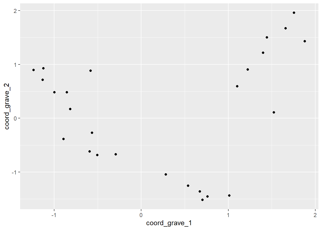

2.2 Table with artefacts - function `tidyr::tibble()`

now it is little bit more complicated, because we need to create a new table for the artefacts. Each row will be one type of artefact and the variables will be their coordinates
tidyr::tibble() creates a “tibble” which is a type of dataframe and works well with tidy data

here, tibble() binds together 2 vectors with the coordinates together with the third vector “artefact”, that consists of artefact names. These names are extracted by colnames() from the names of the columns defined by select()

table_artefacts <- tibble(
  coord_artefact_1,
  coord_artefact_2,
  artefact = df_graves_wide |> 
    select(beaker:spear) |> 
    colnames()
)

head(table_artefacts, 6)

# A tibble: 6 × 3
  coord_artefact_1 coord_artefact_2 artefact  
             <dbl>            <dbl> <chr>     
1           -1.13            0.0601 beaker    
2           -0.211          -0.372  dartpoint 
3           -0.578          -0.331  wristguard
4           -0.954          -0.478  dagger    
5            0.761          -1.89   axe       
6            0.106           0.269  bowl

quick plot

ggplot()+
  geom_point(data = table_artefacts, aes(x=coord_artefact_1, y = coord_artefact_2))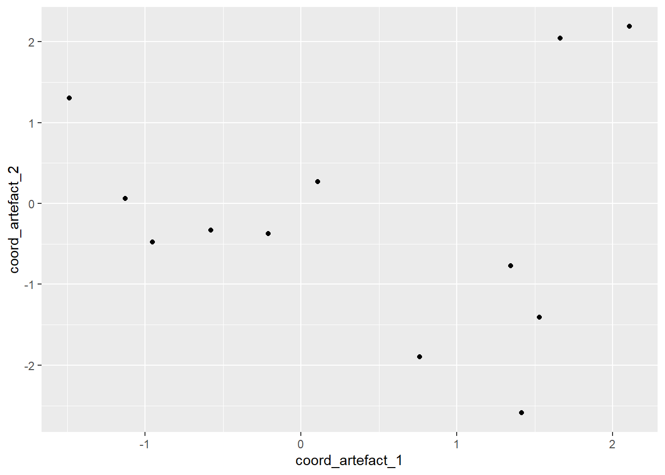

3. and finaly - the `ggplot()`

here, we are visualising each table in a separate geom_point()

ggplot()+
  geom_point(data = table_graves, 
             aes(x = coord_grave_1, y = coord_grave_2, color = dating), 
             shape = 16, size = 2)+
  geom_point(data = table_artefacts, 
             aes(x = coord_artefact_1, y = coord_artefact_2), 
             shape = 17, size = 2)+
  theme_light()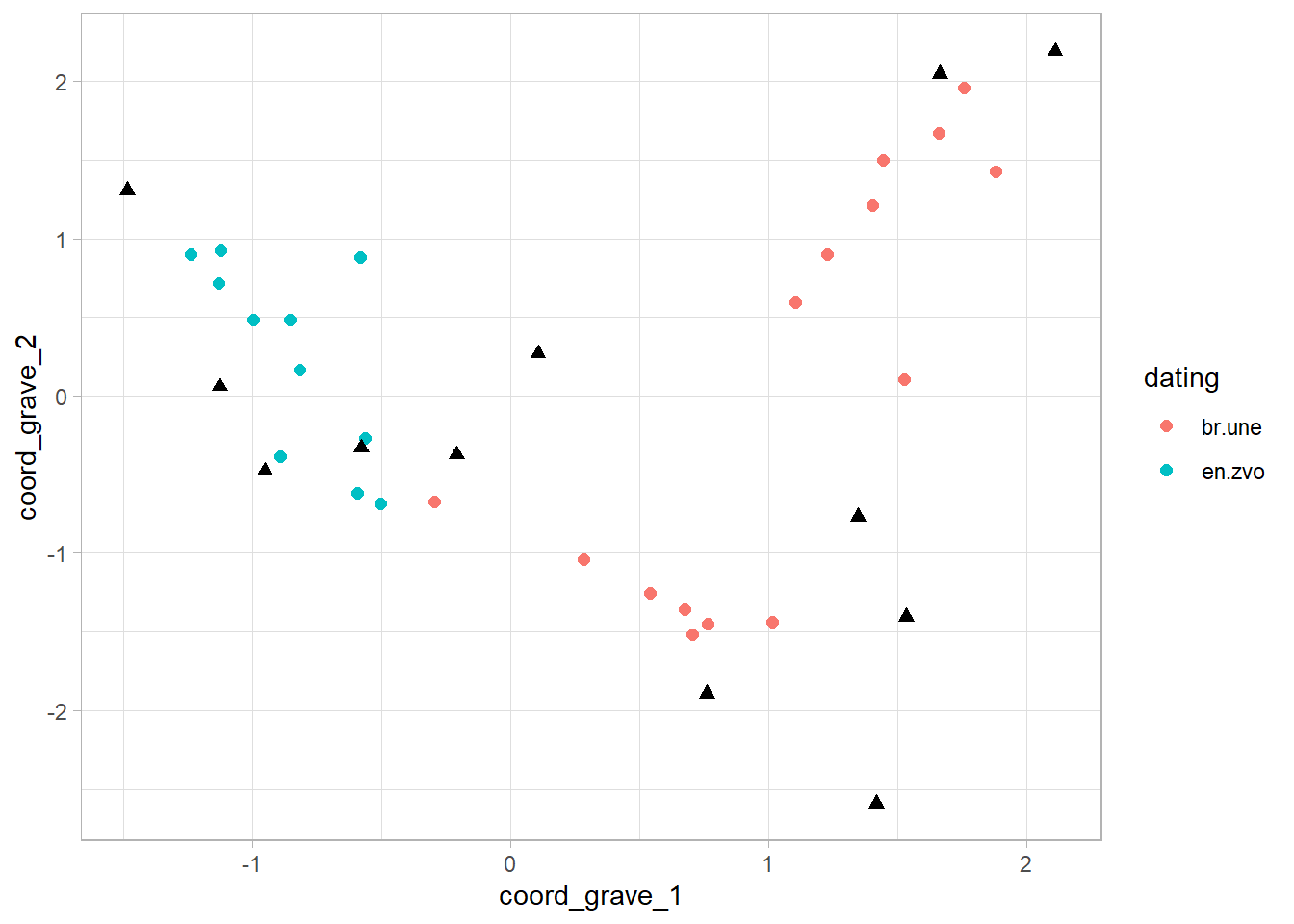

Adjusting the plot

try to identify what is happening in each layer of the ggplot() and play a bit with the settings:

eigenvalue_1 <- 38.58
eigenvalue_2 <- 23.2

ggplot()+
  geom_hline(yintercept = 0,
             color = "gray50",
             linetype = "dashed",
             linewidth = 0.5)+
  geom_vline(xintercept = 0,
             color = "gray50", 
             linetype = "dashed",
             linewidth = 0.5)+
  geom_point(data = table_graves, 
             aes(x = coord_grave_1, y = coord_grave_2, color = dating, fill = dating, shape = sex), 
             alpha = 0.5, 
             size = 2)+
  geom_point(data = table_artefacts, 
             aes(x = coord_artefact_1, y = coord_artefact_2), 
             shape = 4, 
             size = 2)+
  geom_text(data = table_artefacts,
            aes(label = artefact, x=coord_artefact_1, y=coord_artefact_2), 
            vjust = -1.5,
            size = 3)+
  scale_shape_manual(values = c("male" = 22, "female" = 25, "child" = 21))+
  xlim(-1.55, 2.4)+
  ylim(-2.6, 2.6)+
  labs(x = paste0("dimension 1 (", eigenvalue_1," %)"),
       y = paste0("dimension 2 (", eigenvalue_2," %)"),
       title = "Correspondence analysis")+
  theme_light()

Interpretation

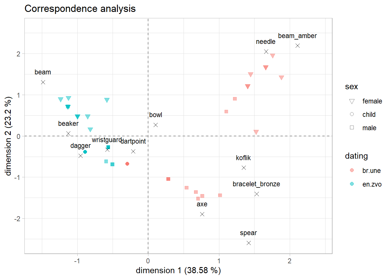
let’s have a look at the plot again and try to answer the research questions:
- are there differences between artefacts in different dating periods?
- are there differences between sexes?
- are there any similar groups of graves?

Introduction

Correspondence analysis (CA) - what is it?

Correspondence analysis (CA) - what do I need?

Contingency table

Doing CA on artificial archaeological data

Prerequisites

Packages:

Data:

Start:

CA - start

Research questions

Tidying data

widening data with tidyr::pivot_wider()

Dealing with NAs

Calculating CA with the function ca()

visualising CA result with plot()

Observing the results structure

Observing the results structure 2

Visualising CA result with ggplot()

Procedure:

1. Extracting coordinates:

2.1 Table with graves

Quick plot:

2.2 Table with artefacts - function tidyr::tibble()

quick plot

3. and finaly - the ggplot()

Adjusting the plot

Interpretation

widening data with `tidyr::pivot_wider()`

Calculating CA with the function `ca()`

visualising CA result with `plot()`

Visualising CA result with `ggplot()`

2.2 Table with artefacts - function `tidyr::tibble()`

3. and finaly - the `ggplot()`