Distances and similarity

Distances and similarity

  • Distance and similarity are more or less opposite concepts.
  • Distance is a numerical measure describing how are two objects (defined by certain variables) different (pairwise distance).
  • Different distance measures exist for different data types.

Distance

  • Scale 0 – \(\infty\)
  • 0 – Two objects with 0 distance between them.
  • \(\infty\) – Two objects with infinite distance.
  • In practice, maximum distance is often 1.
  • Denoted by \(D\) (for distance, or dissimilarity).
  • \(D = 1 - S\)

Similarity

  • Scale 0 – 1
  • 0 – Two objects completely dissimilar (0%).
  • 1 – Two objects competely similar (100%).
  • Denoted by \(S\) (for similarity).
  • \(S = 1 - D\)

Different distance measures

  • Dichotomous variables
    • Symmetrical – Simple matching distance
    • Asymmetrical – Jaccard index (binary distance)
  • Categorical variables
    • Hamming distance
  • Numeric continuous variables
    • Euclidean distance
    • Mahalanobis distance
  • Mixed data sets
    • Gower’s distance

Binary distances

  • For TRUE/FALSE, 1/0, presence/absence (etc.) data

Symmetrical

  • Two presences as match.
  • Two absences as match.

If a trait is present, two objects are more similar. If a trait is absent, two objects are more similar. For example if biological sex is encoded in one variable with 0 for male and 1 for female, it is symmetrical.

  • Simple maching distance

Asymmetrical

  • Two presences as match.
  • Two absences as mismatch.

If a trait is present, two objects are more similar. If a trait is absent in both cases, e.g. undetermined, missing etc., this does not affect similarity. This is more practical in archaeology.

  • Jaccard index, i.e. binary distance

dist(x, method = "binary")

Distance between (continuous) numeric data

  • To remove effects of scale (different units etc.), variables should be scaled (normalized).

Normalization

  • z-score or z-transformation

\[ z = \frac{x - \mu}{\sigma} \]

Euclidean distance

  • Defined for a Cartesian coordinate space.
  • Uses Pythagorean theorem.

\[ d(p, q) = \sqrt{(q_1 - p_1)^2 + (q_2 - p_2)^2} \]

In R…

Normalization:
scale(x, center = TRUE, scale = TRUE)

Euclidean distance:
dist(x, method = "euclidean")

Example – Binary distance

Exercise with the Eneolithic/BA burial ground ( burials.csv).

head(graves0)
  grave_number dating    sex artefact_type artefact_count artefact_material
1          900 en.zvo   male        beaker              3          ceramics
2          901 en.zvo female        beaker              1          ceramics
3          902 en.zvo   male        beaker              1          ceramics
4          903 en.zvo female        beaker              1          ceramics
5          904 en.zvo   male        beaker              1          ceramics
6          905 en.zvo female        beaker              1          ceramics
# artefact counts to presence (TRUE/FALSE)
graves <- graves0 |> 
  mutate(artefact_presence = artefact_count >= 1)
head(graves)
  grave_number dating    sex artefact_type artefact_count artefact_material
1          900 en.zvo   male        beaker              3          ceramics
2          901 en.zvo female        beaker              1          ceramics
3          902 en.zvo   male        beaker              1          ceramics
4          903 en.zvo female        beaker              1          ceramics
5          904 en.zvo   male        beaker              1          ceramics
6          905 en.zvo female        beaker              1          ceramics
  artefact_presence
1              TRUE
2              TRUE
3              TRUE
4              TRUE
5              TRUE
6              TRUE

Table transformation

# long table -> wide table
graves_artefacts <- graves |> 
  tidyr::pivot_wider(
    id_cols = c("grave_number"), 
    names_from = "artefact_type", 
    values_from = "artefact_presence", 
    values_fill = FALSE # fill in missing values with FALSE
  )
head(graves_artefacts)
# A tibble: 6 × 13
  grave_number beaker dartpoint wristguard dagger axe   bowl  beam  beam_amber
         <int> <lgl>  <lgl>     <lgl>      <lgl>  <lgl> <lgl> <lgl> <lgl>     
1          900 TRUE   TRUE      TRUE       TRUE   TRUE  TRUE  FALSE FALSE     
2          901 TRUE   TRUE      TRUE       FALSE  FALSE TRUE  TRUE  FALSE     
3          902 TRUE   TRUE      TRUE       FALSE  FALSE TRUE  FALSE FALSE     
4          903 TRUE   TRUE      TRUE       FALSE  FALSE TRUE  TRUE  FALSE     
5          904 TRUE   TRUE      TRUE       FALSE  FALSE TRUE  FALSE FALSE     
6          905 TRUE   TRUE      TRUE       FALSE  FALSE TRUE  TRUE  FALSE     
# ℹ 4 more variables: koflik <lgl>, bracelet_bronze <lgl>, needle <lgl>,
#   spear <lgl>

Count distance

# matrix with logical variables only
artefacts <- graves_artefacts |> 
  select(where(is.logical)) |> 
  as.matrix()

# add row names to the matrix
rownames(artefacts) <- graves_artefacts$grave_number
artefacts[1:6, 1:6]
    beaker dartpoint wristguard dagger   axe bowl
900   TRUE      TRUE       TRUE   TRUE  TRUE TRUE
901   TRUE      TRUE       TRUE  FALSE FALSE TRUE
902   TRUE      TRUE       TRUE  FALSE FALSE TRUE
903   TRUE      TRUE       TRUE  FALSE FALSE TRUE
904   TRUE      TRUE       TRUE  FALSE FALSE TRUE
905   TRUE      TRUE       TRUE  FALSE FALSE TRUE
# count Jaccard (binary) distance
d <- dist(artefacts, method = "binary", diag = TRUE)

as.matrix(d)[1:6, 1:6]
          900       901       902       903       904       905
900 0.0000000 0.5000000 0.3333333 0.4285714 0.3333333 0.4285714
901 0.5000000 0.0000000 0.3333333 0.1666667 0.3333333 0.1666667
902 0.3333333 0.3333333 0.0000000 0.2000000 0.0000000 0.2000000
903 0.4285714 0.1666667 0.2000000 0.0000000 0.2000000 0.0000000
904 0.3333333 0.3333333 0.0000000 0.2000000 0.0000000 0.2000000
905 0.4285714 0.1666667 0.2000000 0.0000000 0.2000000 0.0000000
  • Result is a distance matrix.
  • It is symmetrical. Lower triangular is the same as upper triangular.
  • On the diagonal, there is distance of the given object to itself, i.e. 0.

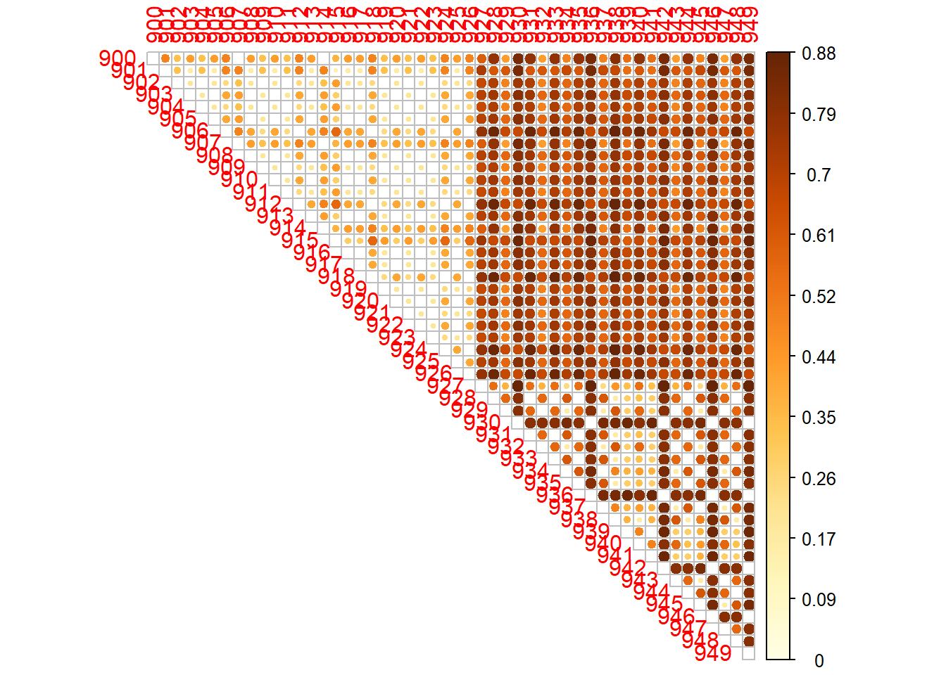
Visualizing distance matrix

  • Package corrplot has a nice way of plotting heat maps.
library(corrplot)

# arg. is.corr set to FALSE, because we are not visualizing correlation matrix
corrplot::corrplot(as.matrix(d), is.corr = FALSE, type = "upper")

Resources

For a much more detailed overview of distance methods, see the tutorial on classification by Schmidt, S. C. et al. DOI: 10.5281/zenodo.6325372 (direct link to a HTML file is here).