Data manipulation with dplyr

Data Transformation

Package

dplyr

Goals

We will learn how to:

select desired variables – select()
rename your variables – rename()
order them from lowest to highest values (or vice versa) – arrange()
filter your data based on different conditions – filter()
calculate different summary statistics such as mean or count – summarise()
add new variables such as percentage – mutate()
work with different functions more effectively – %>%
save your results as comma separated file

Before we begin

load packages here and dplyr (don’t forget to install them firstly, if you haven’t done so yet)
open the project from last lecture (or create a new one if you don’t have it)
create a new script
load data dartpoints.csv into your script
if you are loading data with here function don’t forget to check whether your data and script are in the same folder as your project
create an object called “sipky” from the loaded database (with <-)

library(here)
library(dplyr)
sipky <- read.csv(here("dartpoints.csv"))

Selecting variables

select(dataframe, variable1, variable2)
sometimes you will need to remove variables you don’t need in your work, to have your database more user friendly
for example, you need only variables dealing with major proportions of the dartpoints, but your database have plenty of other variables which are making it difficult to observe, like here:

head(sipky)

  Name Catalog     TARL  Quad Length Width Thickness B.Width J.Width H.Length
1 Darl 41-0322 41CV0536 26/59   42.8  15.8       5.8    11.3    10.6     11.6
2 Darl 35-2946 41CV0235 21/63   40.5  17.4       5.8      NA    13.7     12.9
3 Darl 35-2921 41CV0132 20/63   37.5  16.3       6.1    12.1    11.3      8.2
4 Darl 36-3487 41CV0594 10/54   40.3  16.1       6.3    13.5    11.7      8.3
5 Darl 36-3321 41CV1023 12/58   30.6  17.1       4.0    12.6    11.2      8.9
6 Darl 35-2959 41CV0235 21/63   41.8  16.8       4.1    12.7    11.5     11.0
  Weight Blade.Sh Base.Sh Should.Sh Should.Or Haft.Sh Haft.Or
1    3.6        S       I         S         T       S       E
2    4.5        S       I         S         T       S       E
3    3.6        S       I         S         T       S       E
4    4.0        S       I         S         T       S       E
5    2.3        S       I         S         T       S       E
6    3.0        S       E         I         T       I       C

Selecting variables

to create a new dataframe, simply use function select and define which variables you want to keep

sipky <- select(sipky, Name, Length, Width, Weight)
head(sipky)

  Name Length Width Weight
1 Darl   42.8  15.8    3.6
2 Darl   40.5  17.4    4.5
3 Darl   37.5  16.3    3.6
4 Darl   40.3  16.1    4.0
5 Darl   30.6  17.1    2.3
6 Darl   41.8  16.8    3.0

Renaming variables

renaming your variables with function rename(data, new_name = old_name) can be useful when dealing with complicated code names or different languages
Hint: don’t forget to save object with new variable names by <-

sipky <- rename(sipky,
   typ = Name,
   delka = Length,
   sirka = Width,
   hmotnost = Weight)

head(sipky)

   typ delka sirka hmotnost
1 Darl  42.8  15.8      3.6
2 Darl  40.5  17.4      4.5
3 Darl  37.5  16.3      3.6
4 Darl  40.3  16.1      4.0
5 Darl  30.6  17.1      2.3
6 Darl  41.8  16.8      3.0

Arranging values in ascending order…

here you can order your observations from the lowest to highest (or vice versa). To do so, use function arrange(data, variable)

head(arrange(sipky, delka))

   typ delka sirka hmotnost
1 Darl  30.6  17.1      2.3
2 Darl  31.2  15.6      2.5
3 Darl  32.0  16.0      3.3
4 Darl  32.4  14.5      2.5
5 Darl  33.1  17.4      4.2
6 Darl  33.5  16.6      3.2

…and in descending order

if you want to order the values from higher to smaller just add desc()

head(arrange(sipky, desc(delka)))

         typ delka sirka hmotnost
1 Pedernales 109.5  49.3     28.8
2 Pedernales  84.0  21.2      9.3
3 Pedernales  78.3  28.1     14.8
4 Pedernales  70.4  30.4     13.1
5     Travis  69.0  20.9     11.4
6 Pedernales  67.2  27.1     15.3

Task: What will happen if you will try to order non-numerical variable, but a categorical variable (such as type of the dartpoint)?

Filtering

function filter(data, variable <operator> value) allows you to filter your data based on different conditions, for example minimal weight, type of the dartpoint, etc
logical and mathematical operators: ==, !=, <, >, >=, <=, &, |, etc (use ?dplyr::filter for more details)

here we use > to get only dartpoints with the length higher than 80 cm

filter(sipky, delka > 80)

         typ delka sirka hmotnost
1 Pedernales 109.5  49.3     28.8
2 Pedernales  84.0  21.2      9.3

and here we use == to choose only those dartpoints which are of type “Travis”

filter(sipky, typ == "Travis")

      typ delka sirka hmotnost
1  Travis  56.5  21.1      9.5
2  Travis  54.6  22.4     10.4
3  Travis  46.3  21.3      7.5
4  Travis  57.6  18.9      8.7
5  Travis  49.1  21.4      6.9
6  Travis  64.6  21.5     15.0
7  Travis  69.0  20.9     11.4
8  Travis  40.1  18.4      6.3
9  Travis  41.5  19.2      7.5
10 Travis  46.3  17.9      5.9
11 Travis  39.6  21.5      5.4

alternatively, you can exclude all points of a type “Travis” by negation !=

head(filter(sipky, typ != "Travis"))

   typ delka sirka hmotnost
1 Darl  42.8  15.8      3.6
2 Darl  40.5  17.4      4.5
3 Darl  37.5  16.3      3.6
4 Darl  40.3  16.1      4.0
5 Darl  30.6  17.1      2.3
6 Darl  41.8  16.8      3.0

add & if you want to filter with more than one condition, for example here we will filter all points which are type “Wells” AND are heavier than 10 grams

filter(sipky, typ == "Wells" & hmotnost > 10)

    typ delka sirka hmotnost
1 Wells  65.4  25.1     12.6
2 Wells  58.9  24.4     10.5
3 Wells  63.1  24.7     16.3

Task: instead of & try operator | (OR) and see how the result differs

Filtering based on a vector

you can make your code less complicated when you create vector from desired values and then filter all observations which fall into that vector by using operator %in%

vyber <- c("Pedernales", "Ensor")

head(filter(sipky, typ %in% vyber))

    typ delka sirka hmotnost
1 Ensor  43.5  20.1      4.6
2 Ensor  42.1  20.8      5.4
3 Ensor  42.1  25.1      5.9
4 Ensor  43.1  20.0      5.1
5 Ensor  37.5  21.8      4.7
6 Ensor  55.2  22.5      7.2

Summaries

we already know some functions to calculate basic summaries, for example function mean

mean(sipky$delka)

[1] 49.33077

but if you want to create a new dataframe from calculated statistics, function summarise(data, new_variable = summary_statistics) is much more helpfull
for summary statistics you can use different functions: mean(), median(), sd(), min()…, (use ?summarise for more details)

summarise(sipky, delka_prumer = mean(delka))

  delka_prumer
1     49.33077

you can also calculate more summaries:

summarise(sipky,
    delka_prumer = mean(delka),
    delka_sd = sd(delka),
    delka_min = min(delka),
    delka_max = max(delka),
    pocet = n())

  delka_prumer delka_sd delka_min delka_max pocet
1     49.33077 12.73619      30.6     109.5    91

Grouping

summaries above were applied on whole dataframe. Here we will learn how to calculate summaries for each type of the dartpoint by using group_by(data, variable_to_be_grouped_by)

sipky_typ <- group_by(sipky, typ)

at first sight, you don´t see any differences, but they will be visible after applying function summarise

summarise(sipky_typ, delka_prumer = mean(delka))

# A tibble: 5 × 2
  typ        delka_prumer
  <fct>             <dbl>
1 Darl               39.8
2 Ensor              42.7
3 Pedernales         57.9
4 Travis             51.4
5 Wells              53.1

you can also calculate more summaries at once and use round to remove unnecessary decimals:

summarise(sipky_typ, 
    delka_prumer = round(mean(delka), 1),
    pocet = n())

# A tibble: 5 × 3
  typ        delka_prumer pocet
  <fct>             <dbl> <int>
1 Darl               39.8    28
2 Ensor              42.7    10
3 Pedernales         57.9    32
4 Travis             51.4    11
5 Wells              53.1    10

Task: save the result as a new dataframe “sipky_sum” for later work

sipky_sum <- summarise(sipky_typ, 
    delka_prumer = round(mean(delka), 1),
    pocet = n())

Mutate

function mutate creates a new variable, here we will show how to add variable with percentages
note: sum calculates a total sum of values from chosen variable (in this case - “pocet”)

mutate(sipky_sum,
   procento = pocet/sum(pocet)*100)

# A tibble: 5 × 4
  typ        delka_prumer pocet procento
  <fct>             <dbl> <int>    <dbl>
1 Darl               39.8    28     30.8
2 Ensor              42.7    10     11.0
3 Pedernales         57.9    32     35.2
4 Travis             51.4    11     12.1
5 Wells              53.1    10     11.0

Hint: you can again remove unnecessary decimals by adding round but be careful with the right number of the brackets ()!

mutate(sipky_sum,
   procento = round(pocet/sum(pocet)*100, 0))

# A tibble: 5 × 4
  typ        delka_prumer pocet procento
  <fct>             <dbl> <int>    <dbl>
1 Darl               39.8    28       31
2 Ensor              42.7    10       11
3 Pedernales         57.9    32       35
4 Travis             51.4    11       12
5 Wells              53.1    10       11

Pipe operator

when applying plenty of transformation on one dataset “pipe operator” (%>%) could make your work easier and code shorter and more readable
notice you don´t need to repeat the name of the dataframe into every function arguments, since you already specified it in the begining of the “pipe”

sipky %>% 
  filter(delka > 70) %>%
  arrange(delka)

         typ delka sirka hmotnost
1 Pedernales  70.4  30.4     13.1
2 Pedernales  78.3  28.1     14.8
3 Pedernales  84.0  21.2      9.3
4 Pedernales 109.5  49.3     28.8

More complex summarising with dplyr and pipe

sipky %>% 
  group_by(typ) %>% 
  summarise(
    delka_prum = round(mean(delka), 1),
    hmotnost_prum = round(mean(hmotnost), 1),
    pocet = n()) %>%
  mutate(procento = round(pocet/sum(pocet)*100, 1)) %>% 
  arrange(desc(pocet))

# A tibble: 5 × 5
  typ        delka_prum hmotnost_prum pocet procento
  <fct>           <dbl>         <dbl> <int>    <dbl>
1 Pedernales       57.9          10.6    32     35.2
2 Darl             39.8           4.4    28     30.8
3 Travis           51.4           8.6    11     12.1
4 Ensor            42.7           5.1    10     11  
5 Wells            53.1           8.7    10     11

Visualising your summaries

sipky %>% 
  group_by(typ) %>% 
  summarise(
    delka_prum = mean(delka),
    hmotnost_prum = mean(hmotnost),
    pocet = n()) %>%
  mutate(procento = round(pocet/sum(pocet)*100, 1)) %>% 
  arrange(desc(pocet))

# A tibble: 5 × 5
  typ        delka_prum hmotnost_prum pocet procento
  <fct>           <dbl>         <dbl> <int>    <dbl>
1 Pedernales       57.9         10.6     32     35.2
2 Darl             39.8          4.41    28     30.8
3 Travis           51.4          8.59    11     12.1
4 Ensor            42.7          5.06    10     11  
5 Wells            53.1          8.68    10     11

Visualising your summaries

sipky %>% 
  group_by(typ) %>% 
  summarise(
    delka_prum = mean(delka),
    hmotnost_prum = mean(hmotnost),
    pocet = n()) %>%
  mutate(procento = round(pocet/sum(pocet)*100, 1)) %>% 
  arrange(desc(pocet)) %>% 
  ggplot() +
  aes(x = typ, y = delka_prum) +
  geom_col() +
  labs(title = "Průměrná délka šipky") +
  theme_light()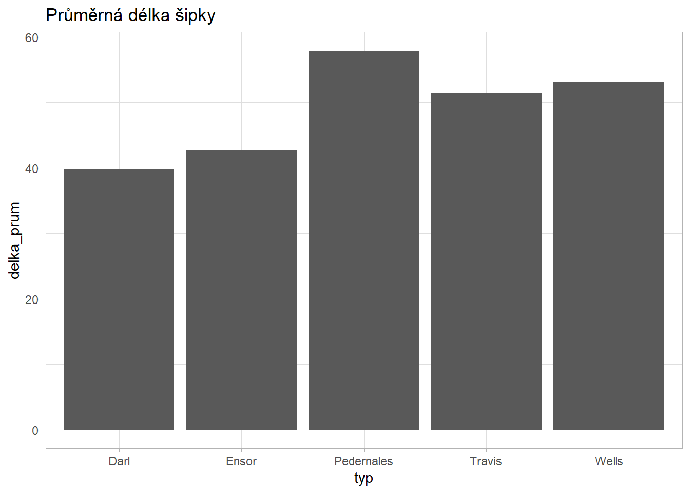

Saving your results

use write.csv for saving your results as a comma separated file

sipky %>% 
  group_by(typ) %>% 
  summarise(
    delka_prum = mean(delka),
    hmotnost_prum = mean(hmotnost),
    pocet = n()) %>%
  mutate(procento = round(pocet/sum(pocet)*100, 1)) %>% 
  arrange(desc(pocet)) %>% 
  write.csv(here("sipky_result.csv"))

or save your summarised data frame as an object and save it later

sipky_result <- sipky %>% 
  group_by(typ) %>% 
  summarise(
    delka_prum = mean(delka),
    hmotnost_prum = mean(hmotnost),
    pocet = n()) %>%
  mutate(procento = round(pocet/sum(pocet)*100, 1)) %>% 
  arrange(desc(pocet))
  
write.csv(sipky_result, here("sipky_result.csv"))

Exercise

Create new a script in your project folder and save.
Load packages necessary for: (a) loading, (b) transformation, and (c) visualization of data.
Load database bacups.csv and save it as an object.
Create a new dataframe having only variables H, RD and Phase.
Try to use pipes %>%.
Rename the variables to height, rimdiameter and phase.
For each phase calculate following summary statistics:
- mean and median vessel height,
- standard deviation of vessel height,
- correlation between height and rim diameter, and
- number of vessels.
Calculate percentage of vessels in each phase.
Arrange the results from highest to lowest mean values.
Save your result as a CSV file
Are height of vessels or rim diameter normally distributed? Why/why not?