Summaries and visualization of distributions

Reflection on the last week

Objectives

At the end of the lecture, you will know how to..

Organize your code in scripts.
Organize your work in projects.
Count and interpret descriptive statics characterizing central tendency of a numeric variable.
Describe spread of a numeric variable.
Read plots for one variable.
Create plots displaying one variable in ggplot2 package.
Understand what type of variation occurs within your variables.

Organize your work in scripts

dartpoints.r

# Analysis of dartpoints data set
# 6. 3. 2024

library(ggplot2)

# data -------------------------------
# read data from CSV
# url: https://petrpajdla.github.io/stat4arch/lect/w02/data/dartpoints.csv
dartpoints <- read.csv("dartpoints2.csv")

# structure --------------------------
colnames(dartpoints)
nrow(dartpoints)
ncol(dartpoints)
str(dartpoints)

mean(dartpoints$Length)

# plots ------------------------------
ggplot(data = dartpoints) +
  aes(x = Length) +
  geom_histogram() +
  labs(x = "Length (cm)", y = "Count")

In RStudio…

Create a new script with Ctrl + Shift + n
Put some basic info on what are you doing at the top.
Use comments # (Ctrl + Shift + c) to write notes.
Comment on the why, not the what.
Divide the code into sections with Ctrl + Shift + r
# Section name ----
Load the packages you use at the top of the script.
RStudio will give you hints, hit Tab to autocomplete function calls.
Execute the current line with Ctr + Enter
Source the whole script with Ctrl + Shift + Enter

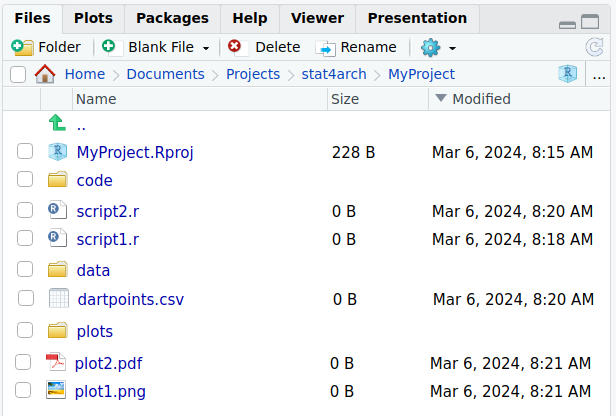
Organize your work in projects

Each project is in a separate directory.
There are subdirectories for different parts of the project.

MyProject/
  code/
    script1.R
    script2.R
  data/
    dartpoints.csv
  plots/
    plot1.png
    plot2.pdf
  MyProject.Rproj

In RStudio go to Files > New Project

Paths

Absolute file path
The file path is specific to a given user.

C:/Documents/MyProject/data/dartpoints.csv

Relative file path
If I am currently in MyProject/ folder:

./data/dartpoints.csv

Package here is here to save the day!

Do not forget to install the package first.
Load it at the top of your script.

# install.packages("here")
library(here)

Function here() will know where the top directory is.

# read data ----
dartpoints <- read_csv(here("data/dartpoints.csv"))

Descriptive Statistics

Characterizing centrality

Mean (průměr)

mean(x)
\[ \overline{x} = \frac{x_1 + x_2 + \cdots + x_n}{n} = \frac{1}{n} (\sum^n_{i=1}x_i) \]

Median (medián)

median(x)
- Robust, minimizes influence of outliers.

What are outliers? (odlehlé hodnoty)

Outliers are data points that significantly differ from other observations.
May indicate a measurement error, an exceptional observation, etc.

Characterizing centrality

Characterizing dispersion and/or spread

Range (rozpětí)

max(x) - min(x) or range(x)

Variance and Standard deviation (rozptyl a směrodatná odchylka)

sd(x)
\[ \sigma = \sqrt{s^2} = \sqrt{\frac{\sum(x_i-\overline{x})^2}{n-1}} \]

Interquartile range (midspread, IQR, kvantil, mezikvartilové rozpětí)

IQR(x)
- Robust, minimizes influence of outliers.

Characterizing dispersion and/or spread

Exercise

Start RStudio.
Create a new project, save it somewhere you can find it.
Use dataset dartpoints2.csv.
Save it in your project directory.
Load the data from the CSV file.
What is the column separator?
How are NAs represented?
Explore the dataset.
Count mean and median weight, how do they differ?
What is the range of the weights?
What is the standard deviation of weights? What does it mean?
Count the IQR. Compare it with standard deviation.
Hints: read.csv2(path, na.strings), str(), colnames(), mean(), median(), range(), sd(), IQR(), summary()

Solution

# dartpoints <- read.csv2(here::here("dartpoints2.csv"), na.strings = "-")
colnames(dartpoints)

 [1] "Name"      "Catalog"   "TARL"      "Quad"      "Length"    "Width"    
 [7] "Thickness" "B.Width"   "J.Width"   "H.Length"  "Weight"    "Blade.Sh" 
[13] "Base.Sh"   "Should.Sh" "Should.Or" "Haft.Sh"   "Haft.Or"

dartpoints$Weight

 [1]  3.6  4.5  3.6  4.0  2.3  3.0  3.9  6.2  5.1  2.8  2.5  4.8  3.2  3.8  4.5
[16]  4.4  2.5  2.3  4.2  3.3  3.6  7.4  5.6  4.8  7.8  9.2  6.2  4.3  4.6  5.4
[31]  5.9  5.1  4.7  7.2  2.5  3.9  4.1  7.2 10.7 12.5 13.4 11.1  7.2 28.8 13.9
[46]  9.4  5.3  7.9  7.3 12.2  9.3 11.1 14.8 10.7 11.1 12.3 13.1  6.1  9.2  9.4
[61]  6.7 15.3 15.1  4.6  4.3 11.6 10.5  6.8  9.1  9.4  9.5 10.4  7.5  8.7  6.9
[76] 15.0 11.4  6.3  7.5  5.9  5.4  9.5  5.4  7.1  9.7 12.6 10.5  5.6  4.9  5.2
[91] 16.3

mean(dartpoints$Weight)

[1] 7.642857

median(dartpoints$Weight)

[1] 6.8

max(dartpoints$Weight) - min(dartpoints$Weight) # or range(dartpoints$Weight)

[1] 26.5

sd(dartpoints$Weight)

[1] 4.207088

IQR(dartpoints$Weight)

[1] 5.5

summary(dartpoints$Weight)

   Min. 1st Qu.  Median    Mean 3rd Qu.    Max. 
  2.300   4.550   6.800   7.643  10.050  28.800

Brainstorming

Why do we visualize data?
What elements does a good graph contain?
How are these elements called?

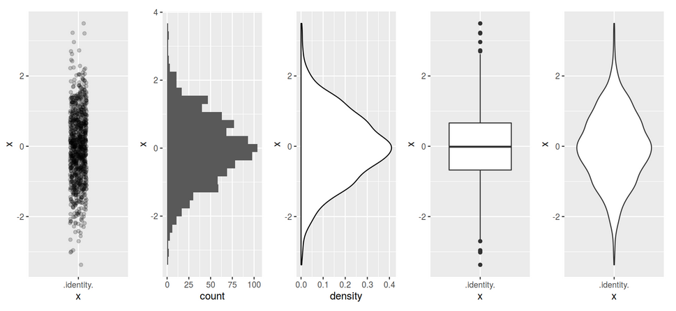
Plots for one variable

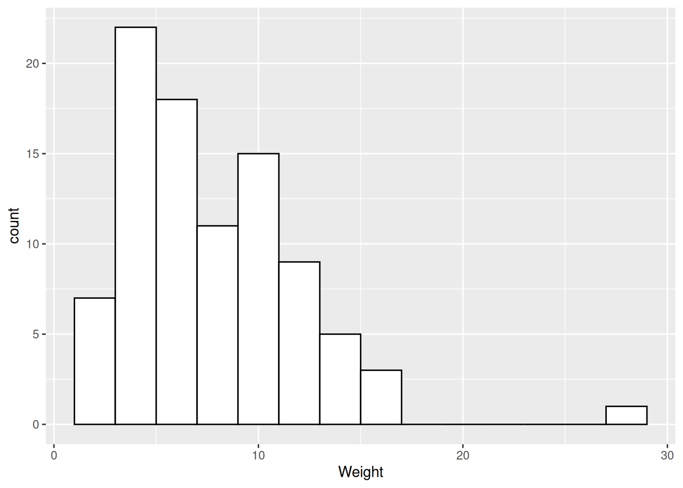
Histogram

Distribution of values of a quantitative variable.

Distribution of dart point weights.

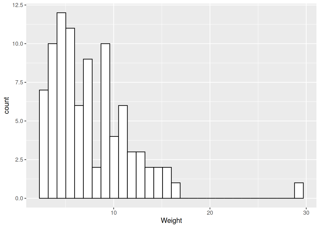
Histogram

Distribution of values of a quantitative variable.

Distribution of dart point weights, one column (bin) equals 2 g.

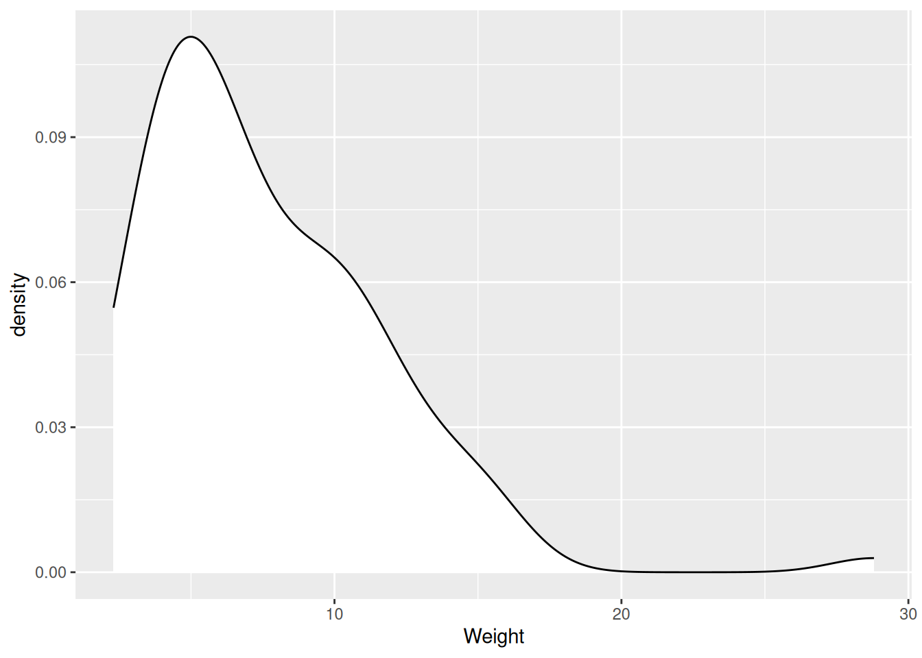
Density plot

Distribution of values of a quantitative variable.

Distribution of dart point weights.

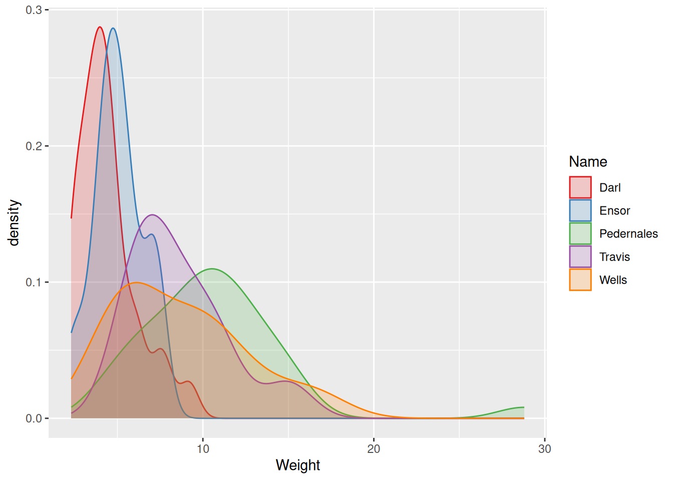
Density plot

Distribution of values of a quantitative variable, great for comparisons.

Distribution of different types of dart points by weight.

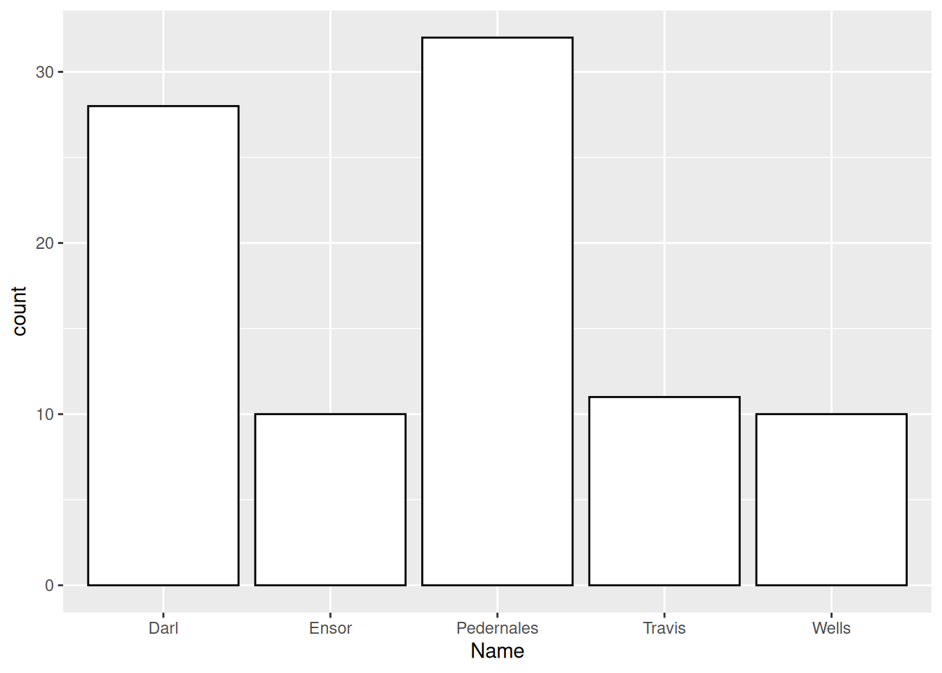
Bar chart

Distribution of values of a qualitative variable.

Distribution of types of dart points.

Plots in ggplot2 package

1install.packages("ggplot2")

2library(ggplot2)

3ggplot(data = <your data frame>) +
4  aes(x = <variable to be mapped to axis x>) +
5  geom_<geometry>()

1: Install the package ggplot2, do this only once.
2: Load the package from the library of installed packages, do this for every new script.
(Calls to library() function are usually written at the top of the script.)
3: Function ggplot() takes the data frame as an argument.
4: Function aes() serves to map aesthetics (axis x and y, colors etc.) to different variables from your data frame.
5: Functons with geom_ prefix are geometries, ie. types of plots to draw.

Geoms for one variable:

geom_histogram()
geom_density()
geom_bar()

Layers of ggplot2

ggplot(data = dartpoints)

Layers of ggplot2

ggplot(data = dartpoints) +
  aes(x = Name)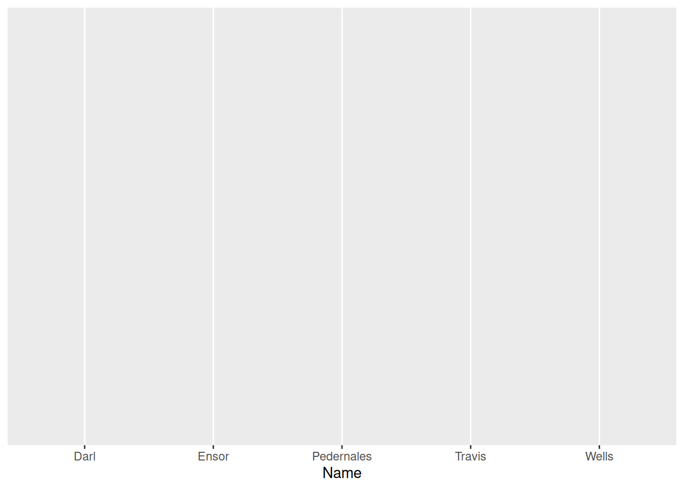

Layers of ggplot2

ggplot(data = dartpoints) +
  aes(x = Name) +
  geom_bar()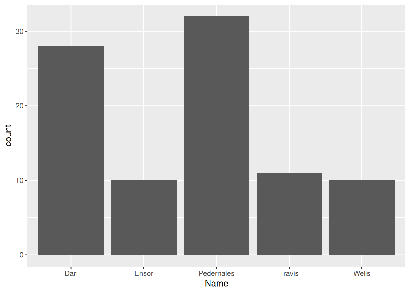

Bar chart

ggplot(data = dartpoints) +
  aes(x = Name) + 
  geom_bar()

Bar chart

ggplot(data = dartpoints) +
  aes(x = Name, color = Name) + 
  geom_bar()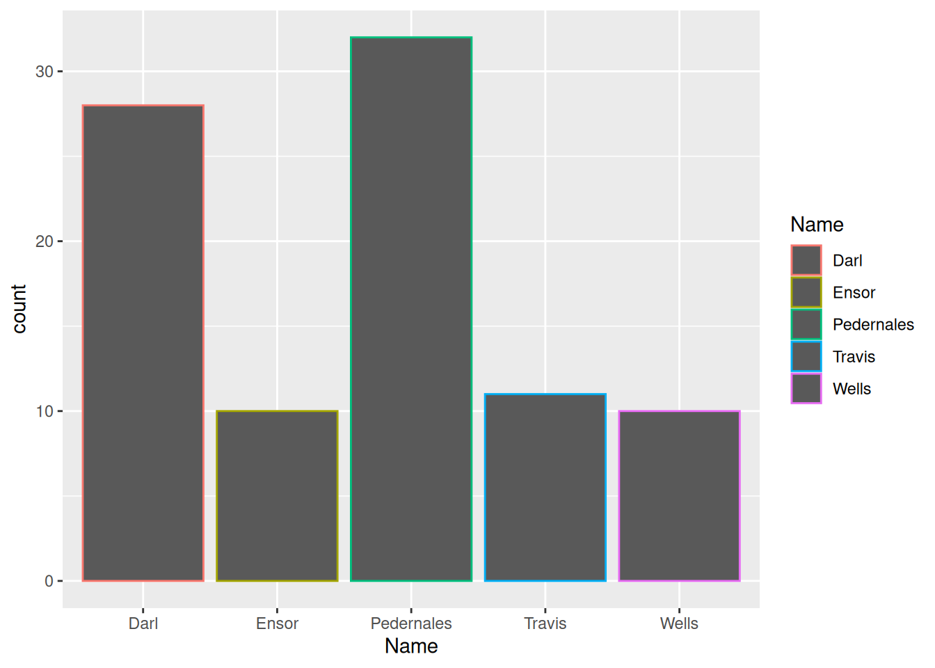

Bar chart

ggplot(data = dartpoints) +
  aes(x = Name, color = Name, fill = Name) + 
  geom_bar()

Bar chart

ggplot(data = dartpoints) + 
  aes(x = Name, fill = Name) + 
  geom_bar(color = "black")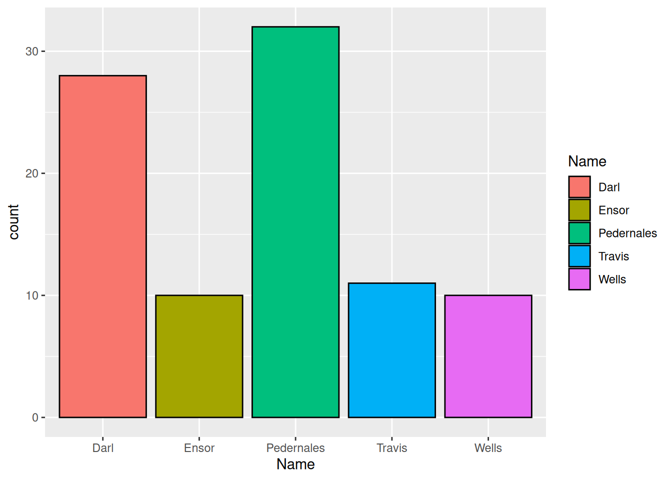

Histogram

ggplot(dartpoints) +
  aes(x = Length) +
  geom_histogram()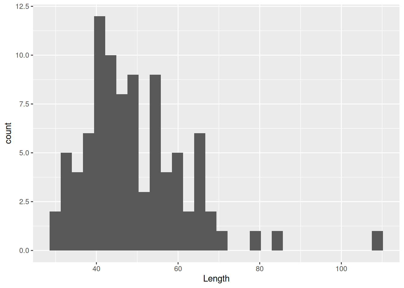

Histogram

ggplot(dartpoints) +
  aes(x = Length) +
  geom_histogram(binwidth = 5)

Histogram

ggplot(dartpoints) +
  aes(x = Length) +
  geom_histogram(binwidth = 5, color = "black")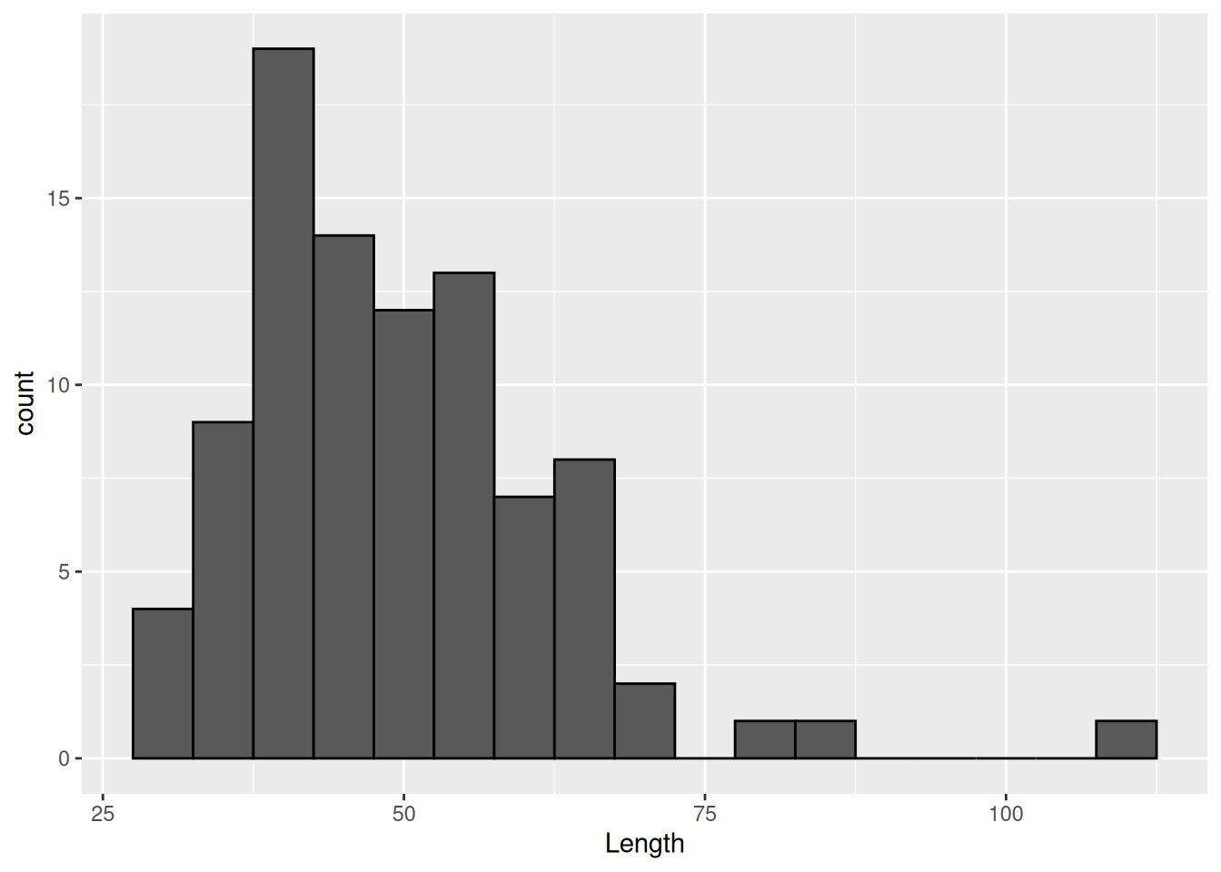

Histogram

ggplot(dartpoints) +
  aes(x = Length) +
  geom_histogram(binwidth = 5, color = "black", fill = "white")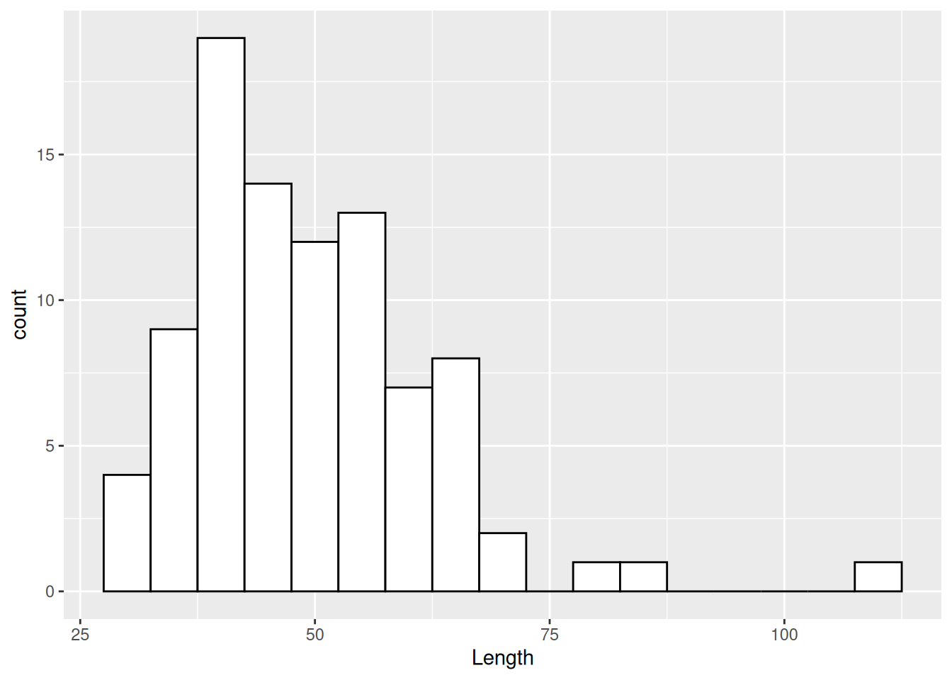

Density plot

ggplot(dartpoints) +
  aes(x = Length) + 
  geom_density()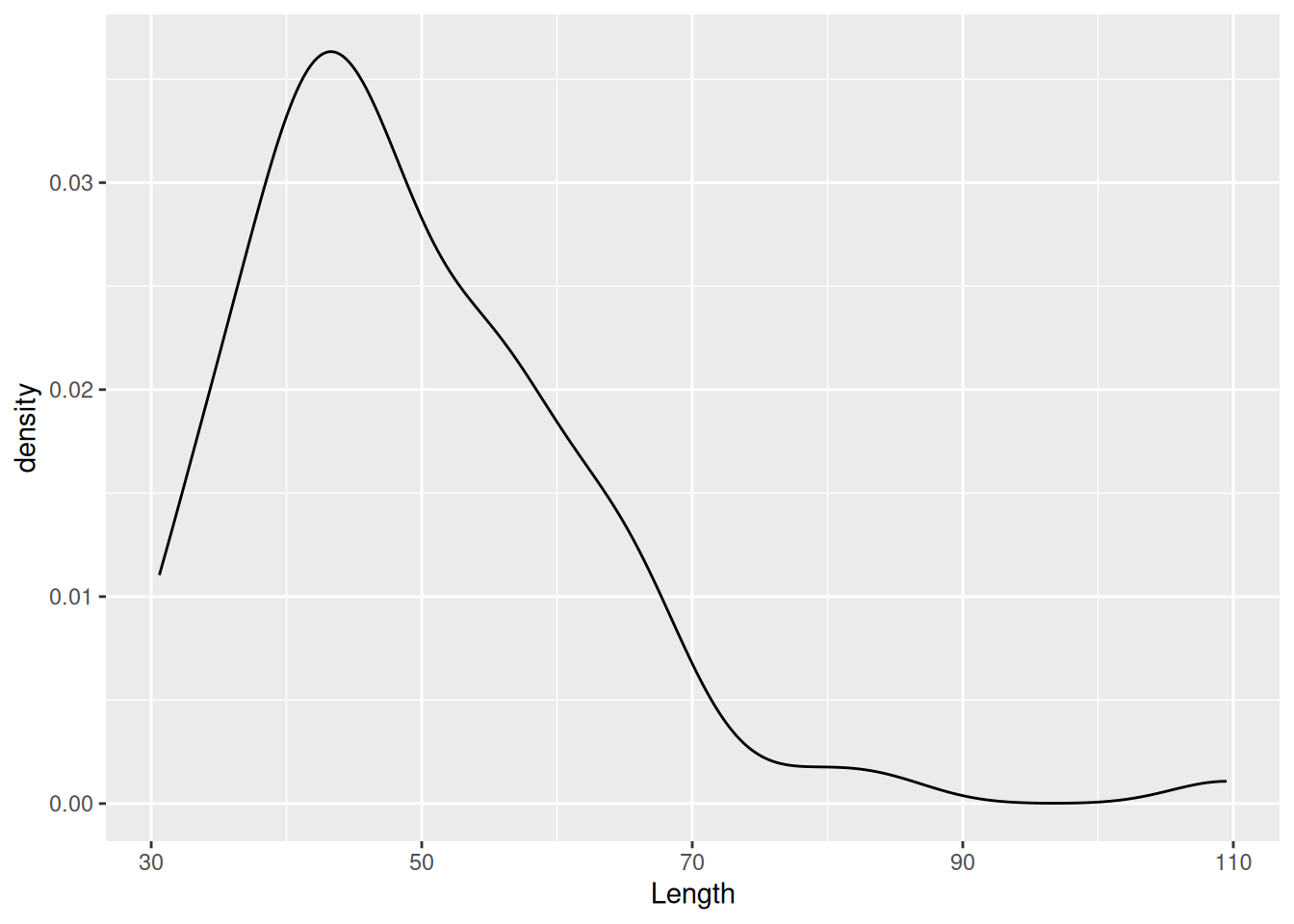

Density plot

ggplot(dartpoints) +
  aes(x = Length, color = Name) + 
  geom_density()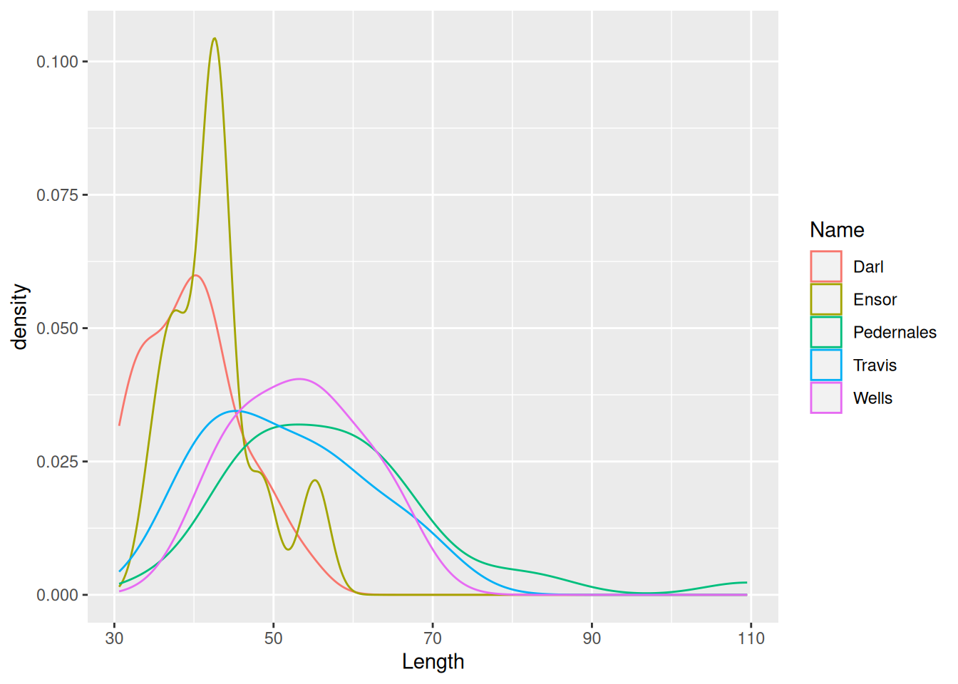

Density plot

ggplot(dartpoints) +
  aes(x = Length, color = Name, fill = Name) + 
  geom_density()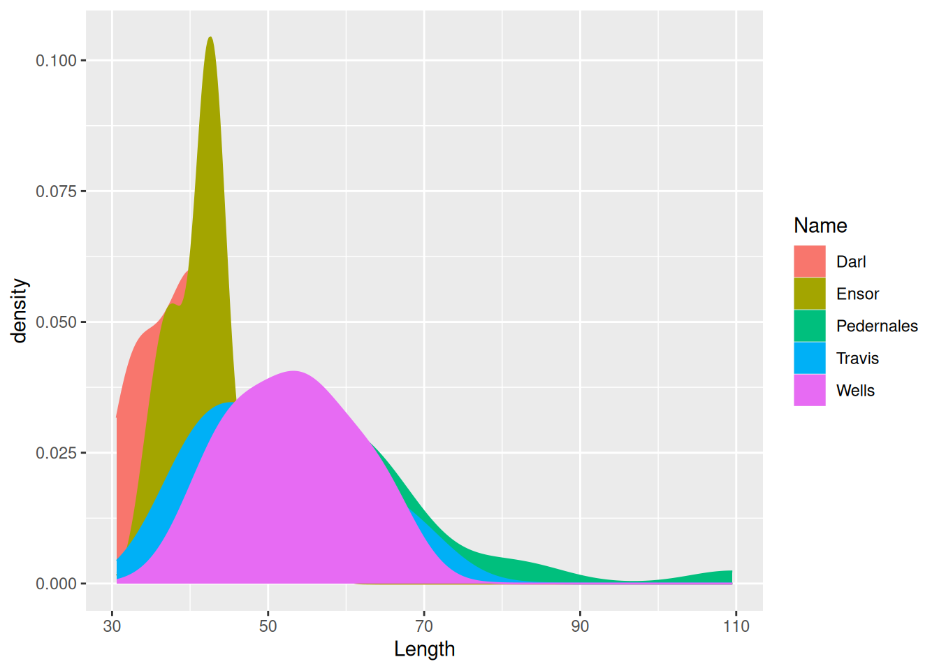

Density plot

ggplot(dartpoints) + 
  aes(x = Length, color = Name, fill = Name) + 
  geom_density(alpha = 0.4)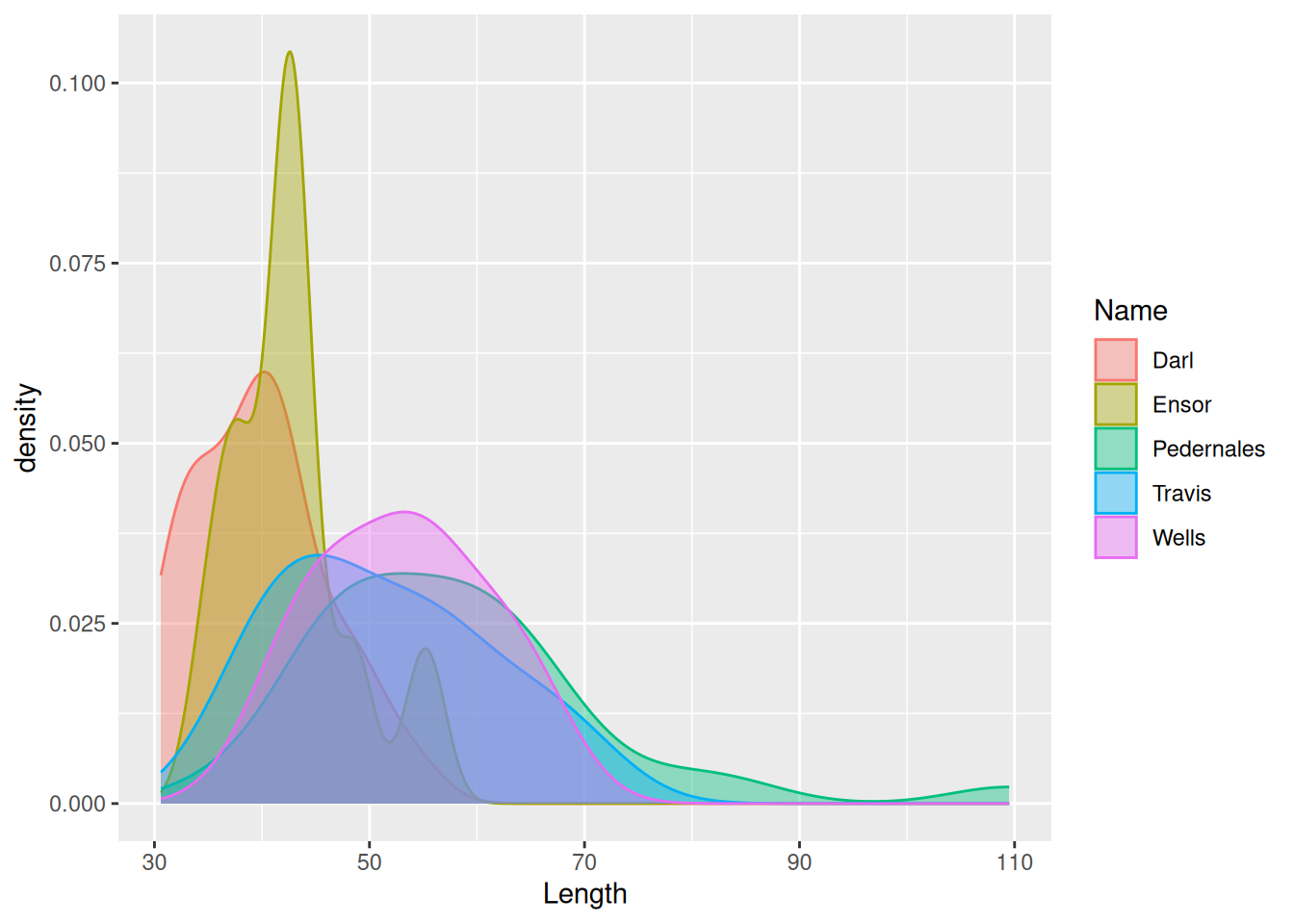

Labels

ggplot(dartpoints) +
  aes(x = Length) +
  geom_histogram(binwidth = 5, color = "black", fill = "white")

Labels

ggplot(dartpoints) +
  aes(x = Length) +
  geom_histogram(binwidth = 5, color = "black", fill = "white") +
  labs(x = "Length (cm)", y = "Count")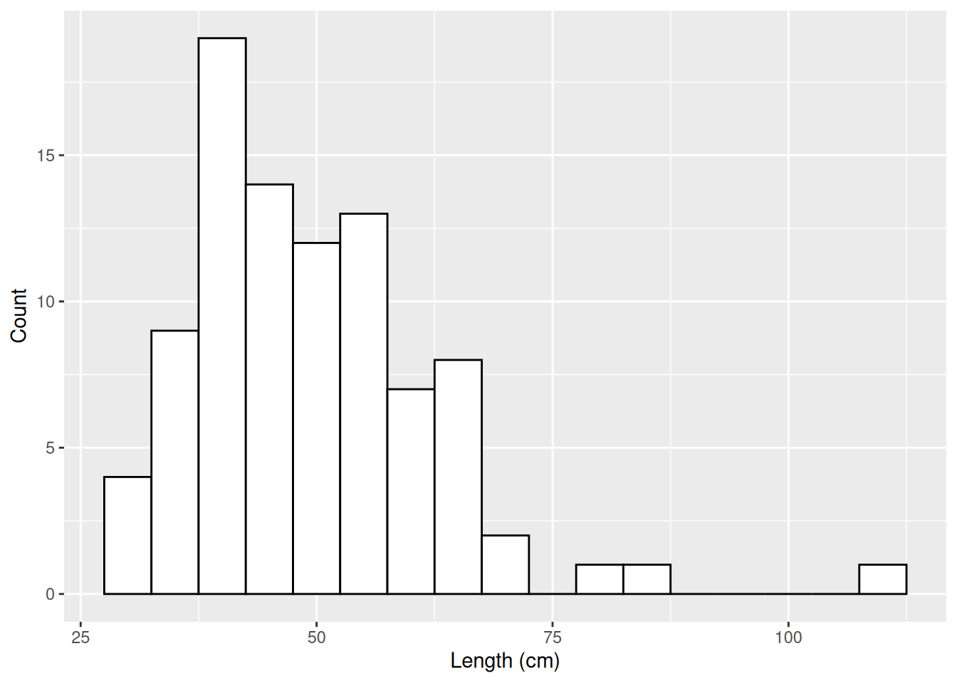

Labels

ggplot(dartpoints) +
  aes(x = Length) +
  geom_histogram(binwidth = 5, color = "black", fill = "white") +
  labs(x = "Length (cm)", y = "Count",
       title = "Histogram of dart point lengths")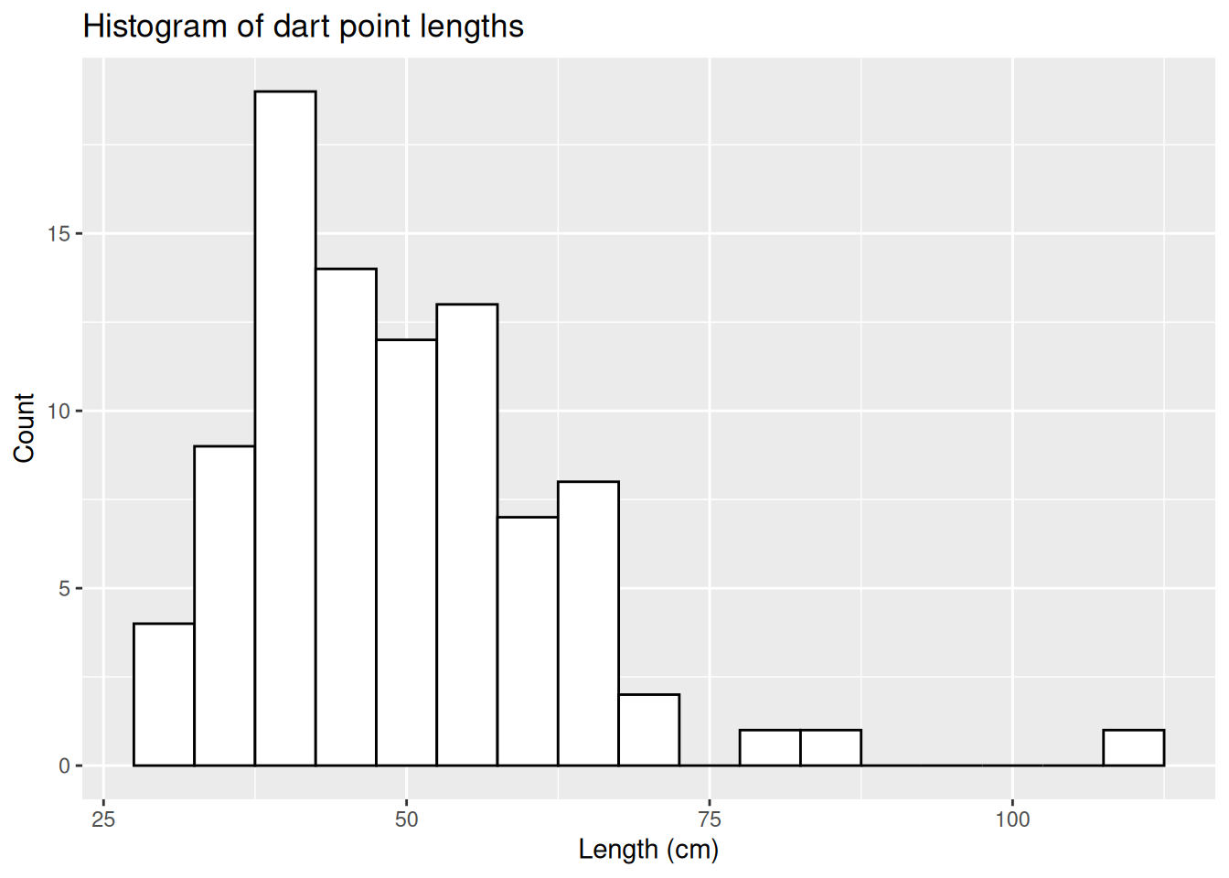

Labels

ggplot(dartpoints) +
  aes(x = Length) +
  geom_histogram(binwidth = 5, color = "black", fill = "white") +
  labs(x = "Length (cm)", y = "Count",
       title = "Histogram of dart point lengths", 
       caption = "Data adapted from archdata R package, Carlson 2017")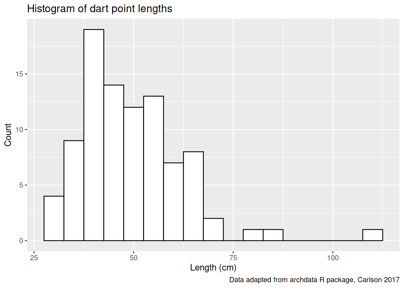

Reflection on the last week

Objectives

Organize your work in scripts

Organize your work in projects

Paths

Descriptive Statistics

Characterizing centrality

Mean (průměr)

Median (medián)

What are outliers? (odlehlé hodnoty)

Characterizing centrality

Characterizing dispersion and/or spread

Range (rozpětí)

Variance and Standard deviation (rozptyl a směrodatná odchylka)

Interquartile range (midspread, IQR, kvantil, mezikvartilové rozpětí)

Characterizing dispersion and/or spread

Exercise

Solution

Brainstorming

Plots for one variable

Histogram

Histogram

Density plot

Density plot

Bar chart

Plots in ggplot2 package

Layers of ggplot2

Layers of ggplot2

Layers of ggplot2

Bar chart

Bar chart

Bar chart

Bar chart

Histogram

Histogram

Histogram

Histogram

Density plot

Density plot

Density plot

Density plot

Labels

Labels

Labels

Labels

Exercises

Assignments

Optional