| datace | ID | pohlavi | nadoby | sipy | cu_dycka | spondyl | kopytovity_klin | desticka | zrnoterka |
|---|---|---|---|---|---|---|---|---|---|
| ne.lin | 1 | F | 4 | 0 | 0 | 5 | 4 | 0 | 1 |
| ne.lin | 2 | M | 3 | 1 | 0 | 2 | 5 | 0 | 0 |
| en.zvo | 3 | F | 7 | 3 | 3 | 0 | 0 | 2 | 0 |
| ne.lin | 4 | F | 2 | 0 | 0 | 4 | 4 | 0 | 1 |
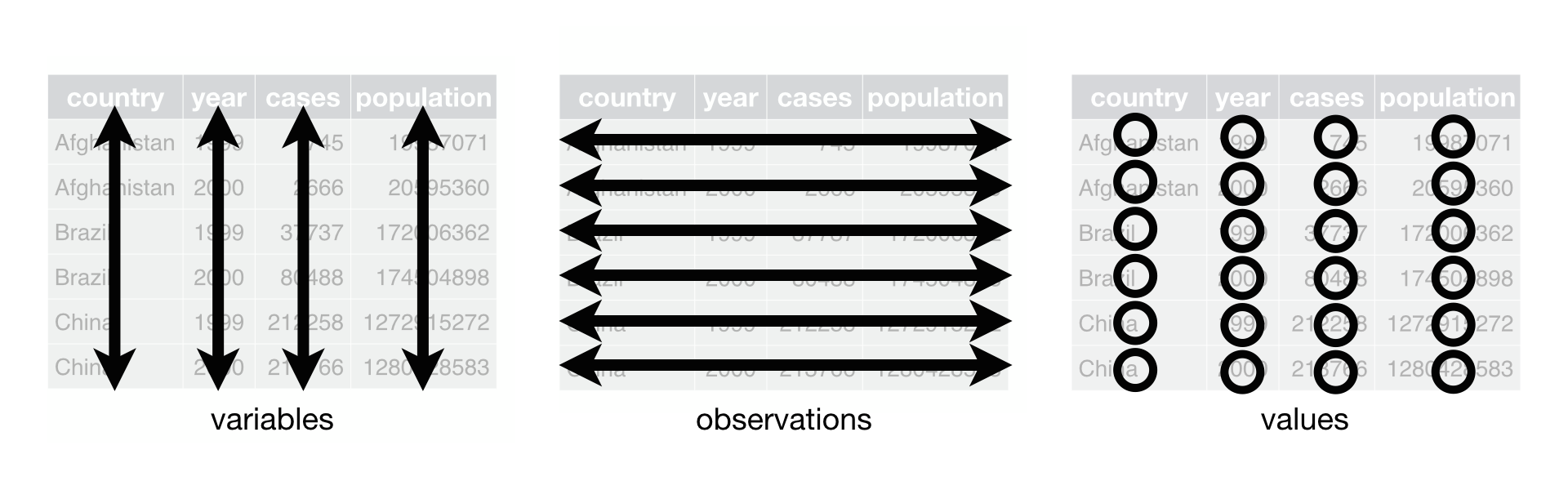
Long table and wide table transformations
You probably still remember the fictional burial site we have been analysing last class with correspondence analysis. Here we have it back again, with two more variables, ID and sex:
You can see that there are three variables describing the grave itself (datace, ID, pohlavi) and rest of the columns are combining two variables in one cell. One variable is the type of a artefakt and other the number of these artefacts.
And if you remember tidy data principles - one object in one in one row, one variable in one column and one value in one cell - you can already feel that we have a problem here.
Wide table
| datace | ID | pohlavi | nadoby | sipy | cu_dycka | spondyl | kopytovity_klin | desticka | zrnoterka |
|---|---|---|---|---|---|---|---|---|---|
| ne.lin | 1 | F | 4 | 0 | 0 | 5 | 4 | 0 | 1 |
| ne.lin | 2 | M | 3 | 1 | 0 | 2 | 5 | 0 | 0 |
| en.zvo | 3 | F | 7 | 3 | 3 | 0 | 0 | 2 | 0 |
| ne.lin | 4 | F | 2 | 0 | 0 | 4 | 4 | 0 | 1 |
This type of dataframe is sometimes called wide table - it has plenty of variables in one row.
It is useful for some analysis such as correspondence analysis, but for others it is not. For example, without major manipulations with columns, it is impossible to plot the number of each artefakt in ggplot, because we don’t have one single variable to plot on x axis.
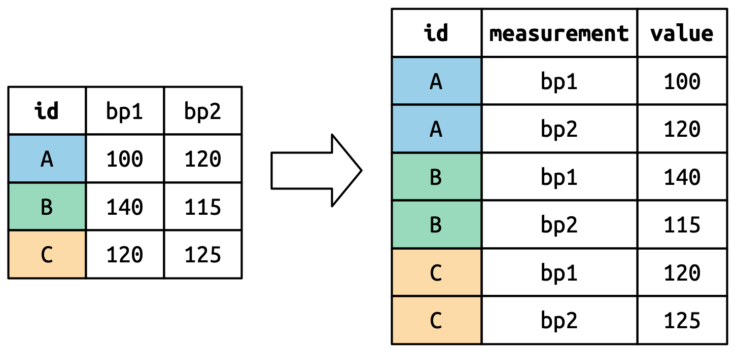
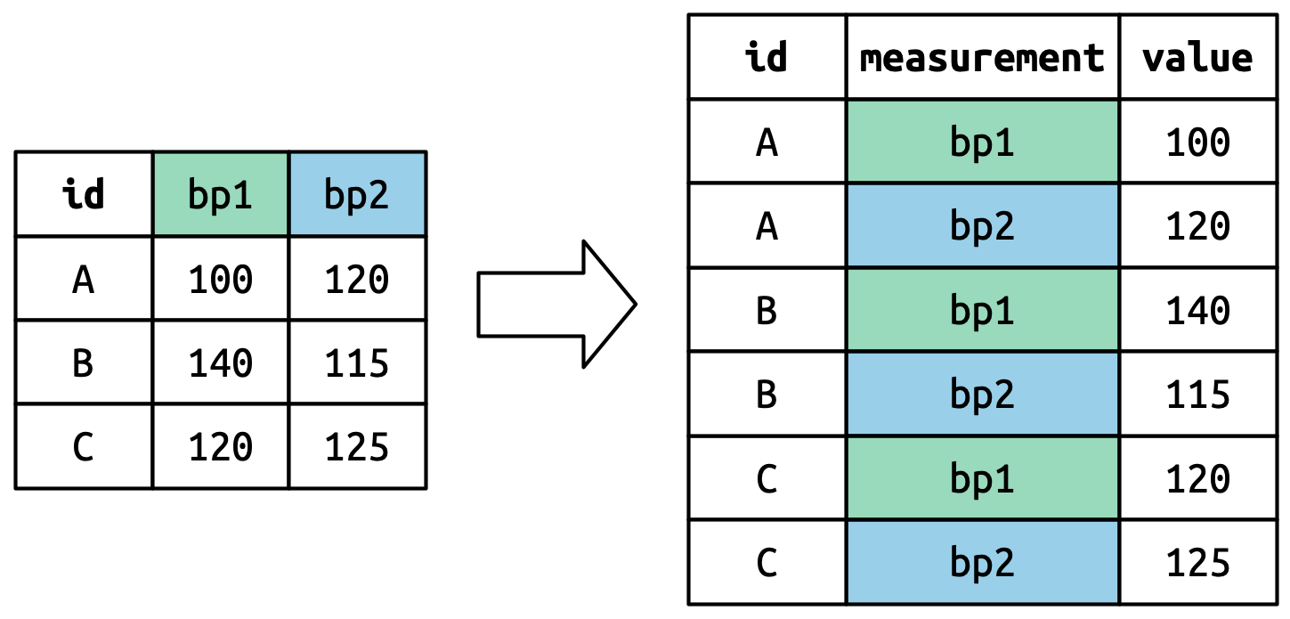
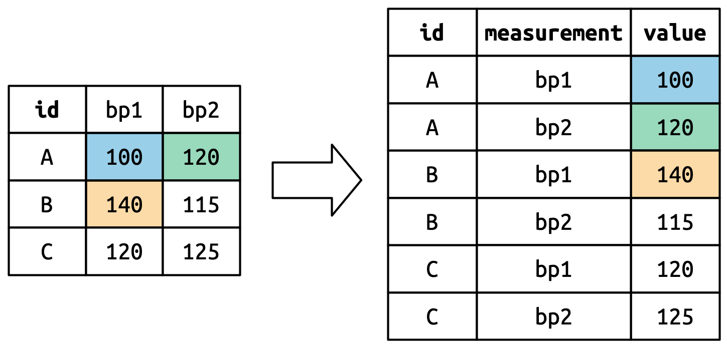
In order to do so, you have to transform wide table to a long table in a way that in one cell there will be only one value of only one variable.
Long table - basic principles
Long table - how to do it in R
Package:
library(dplyr)Function: pivot_longer
pohrebiste_long <- pohrebiste %>%
  pivot_longer(
    cols = c("nadoby", "sipy", "cu_dycka", "spondyl", "kopytovity_klin", "desticka", "zrnoterka"),
    names_to = "artefakt",
    values_to = "pocet"
  )
head(pohrebiste_long, 10)
# A tibble: 10 × 5
datace ID pohlavi artefakt pocet
<chr> <int> <chr> <chr> <dbl>
1 ne.lin 1 F nadoby 4
2 ne.lin 1 F sipy 0
3 ne.lin 1 F cu_dycka 0
4 ne.lin 1 F spondyl 5
5 ne.lin 1 F kopytovity_klin 4
6 ne.lin 1 F desticka 0
7 ne.lin 1 F zrnoterka 1
8 ne.lin 2 M nadoby 3
9 ne.lin 2 M sipy 1
10 ne.lin 2 M cu_dycka 0Quick plot
Now you know what to plot on x axis (artefakt) and what to plot on y axis (pocet) so let’s have one very basic plot:
ggplot(pohrebiste_long, aes(x=artefakt, y=pocet))+
  geom_col()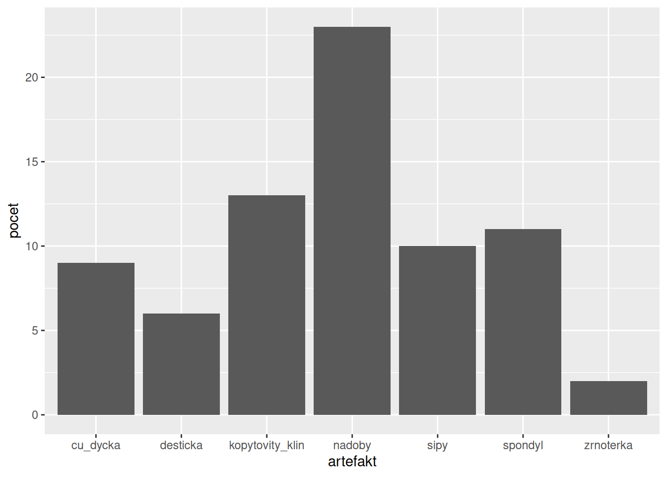
More fancy
And now do it more fancier and add more variables:
ggplot(pohrebiste_long, aes(x=artefakt, y=pocet, fill = pohlavi))+
  geom_col()+
  labs(x="typ artefaktu", y="počet")+
  scale_x_discrete(guide = guide_axis(n.dodge = 2))+
  theme_light()
Oh my, relative values!
ggplot(pohrebiste_long, aes(x=artefakt, y=pocet, fill = pohlavi))+
  geom_col(position = "fill")+
  labs(x="typ artefaktu", y="počet")+
  scale_x_discrete(guide = guide_axis(angle = 30))+
  theme_light()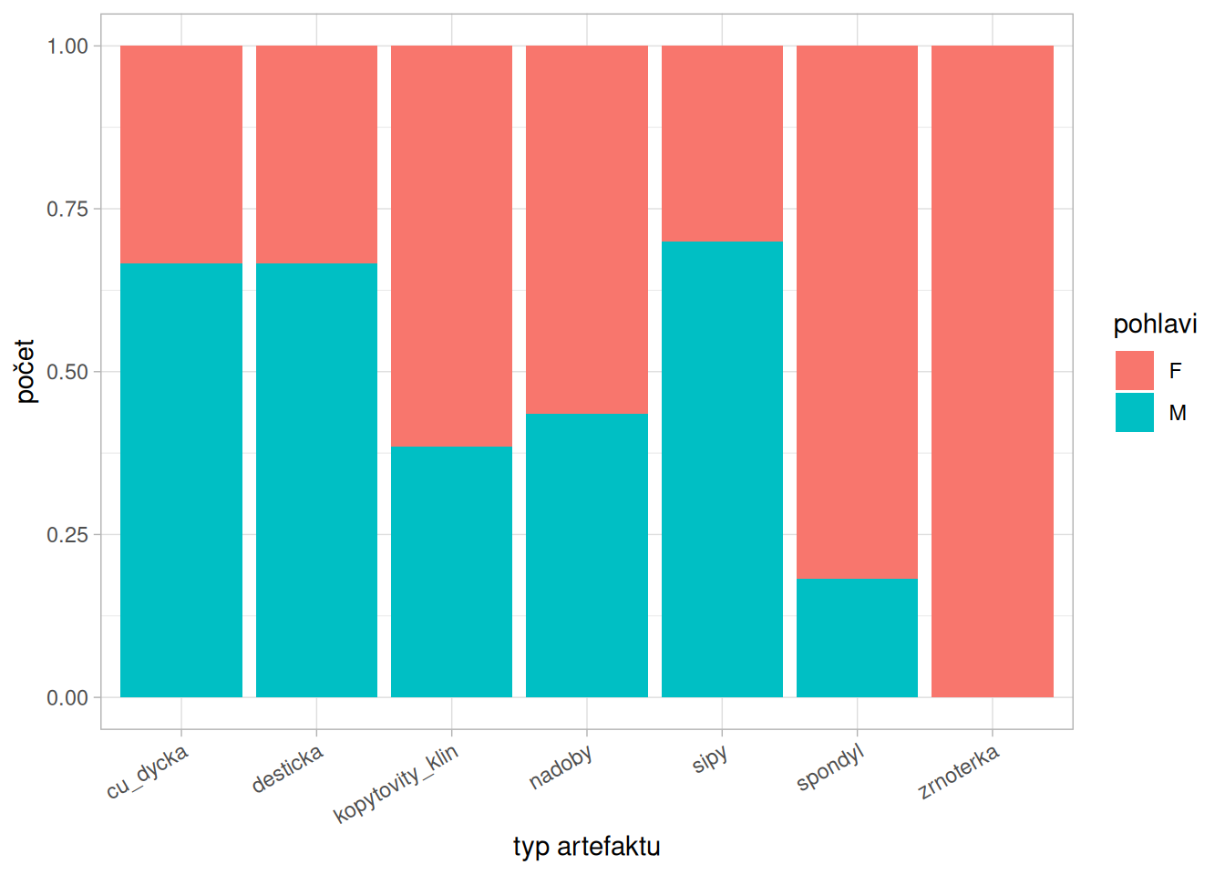
OMG, even two plots!
ggplot(pohrebiste_long, aes(x=artefakt, y=pocet, fill = pohlavi))+
  geom_col()+
  facet_wrap(~pohlavi)+
  labs(x="typ artefaktu", y="počet")+
  scale_x_discrete(     guide = guide_axis(angle = 30))+
  theme_light()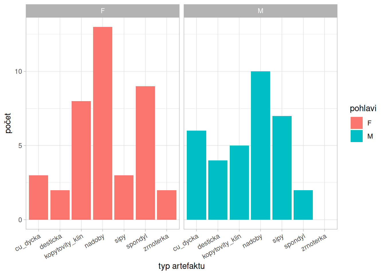
But what if I want to see the numbers for each bar?
Well, it is possible, but we will need some coding:
- first, we need to calculate sum values for each sex and artefakt and to do so, we will use good old dplyr functions:
sum_artefakt <- pohrebiste_long %>%
  group_by(artefakt, pohlavi) %>%
  summarise(pocet_artefaktu=sum(pocet))
head(sum_artefakt, 6)
# A tibble: 6 × 3
# Groups: artefakt [3]
artefakt pohlavi pocet_artefaktu
<chr> <chr> <dbl>
1 cu_dycka F 3
2 cu_dycka M 6
3 desticka F 2
4 desticka M 4
5 kopytovity_klin F 8
6 kopytovity_klin M 5Then
Then we can make the same plot as earlier but now we can add there a new layer with text from the summary table we just created:
ggplot(pohrebiste_long, aes(x=artefakt, y=pocet, fill = pohlavi))+
  geom_bar(stat="identity")+
  geom_text(data=sum_artefakt, aes(label = pocet_artefaktu, x = artefakt, y=pocet_artefaktu), position = position_stack(vjust = 0.5), color = "white")+
  scale_x_discrete(guide = guide_axis(n.dodge = 2))+
  labs(x="typ artefaktu", y="počet")+
  theme_light()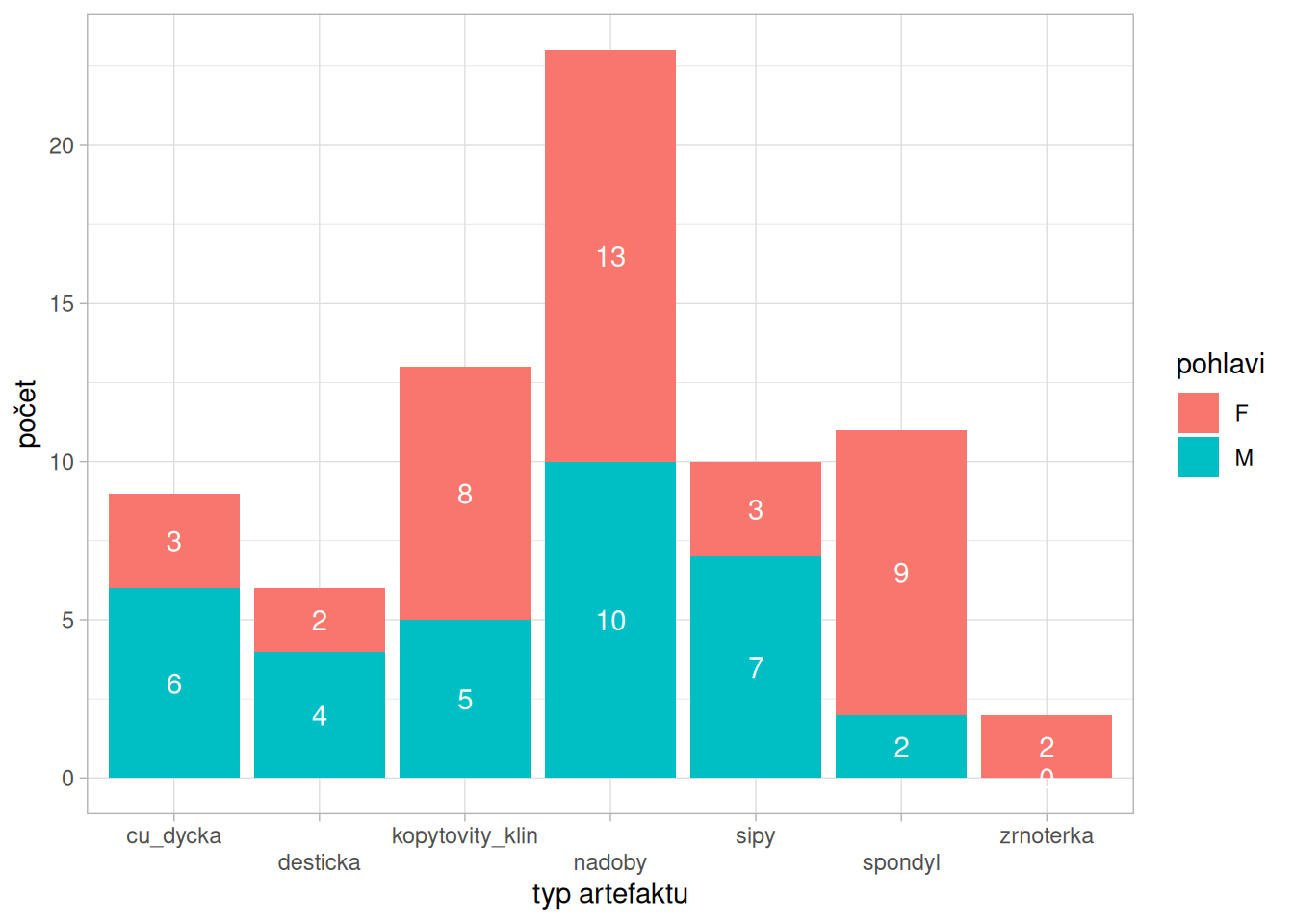
Notice that we are here working with two different (but related) data frames. One is for bar plots and second for text values.