ggplot(dartpoints) + aes(x = Length) + geom_density()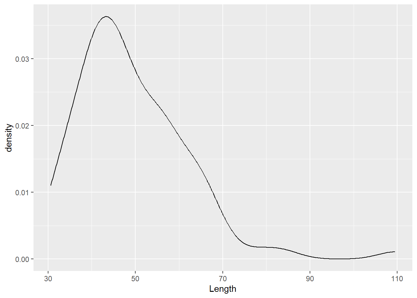
You know how to do the basics:
Some additions…
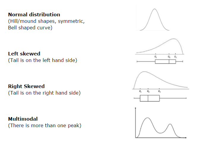
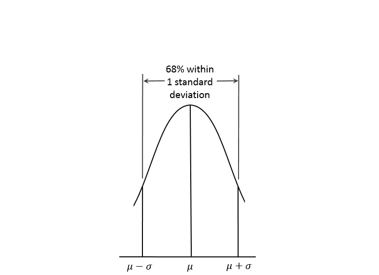
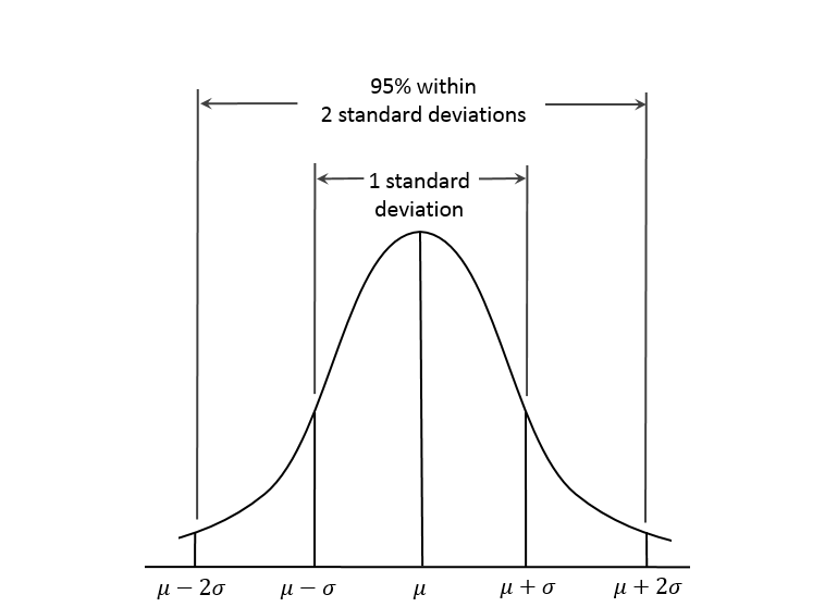
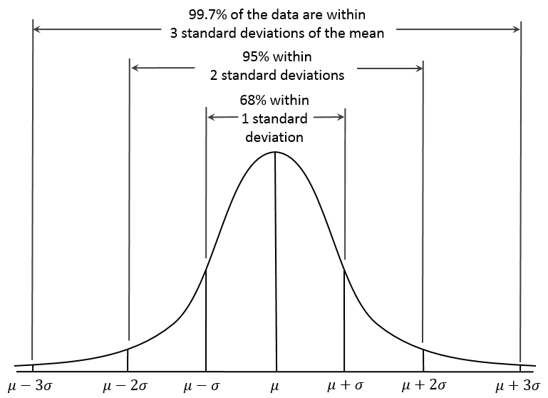
bell-shaped curve, Gaussian distribution
qqnorm() or ggplot(data) + aes(sample = x) + stat_qq()shapiro.text()ggplot(dartpoints) + aes(x = Length) + geom_density()
ggplot(dartpoints) + aes(x = Thickness) + geom_density()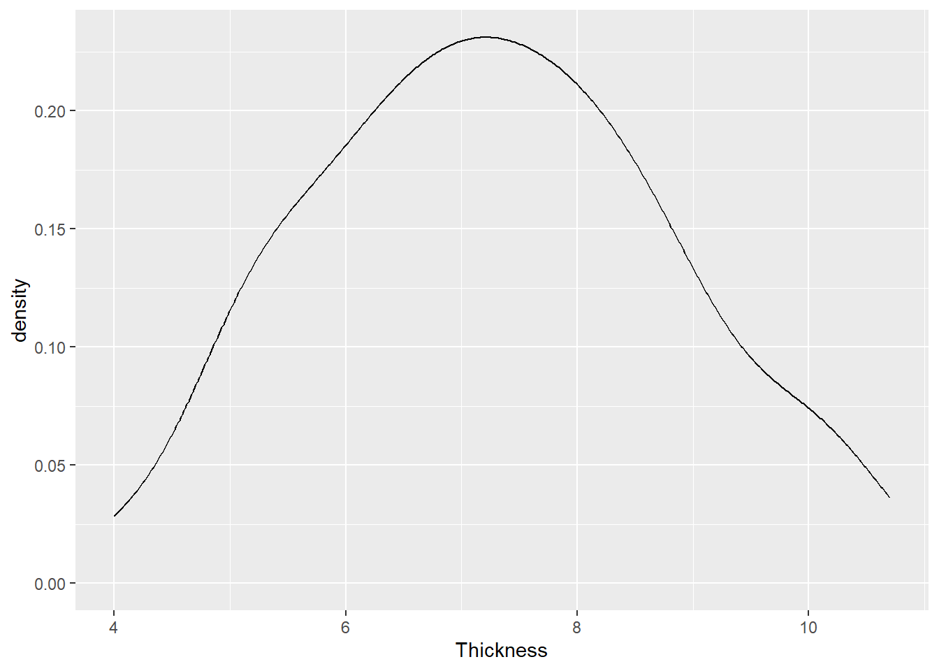
ggplot(dartpoints) + aes(sample = Length) + stat_qq()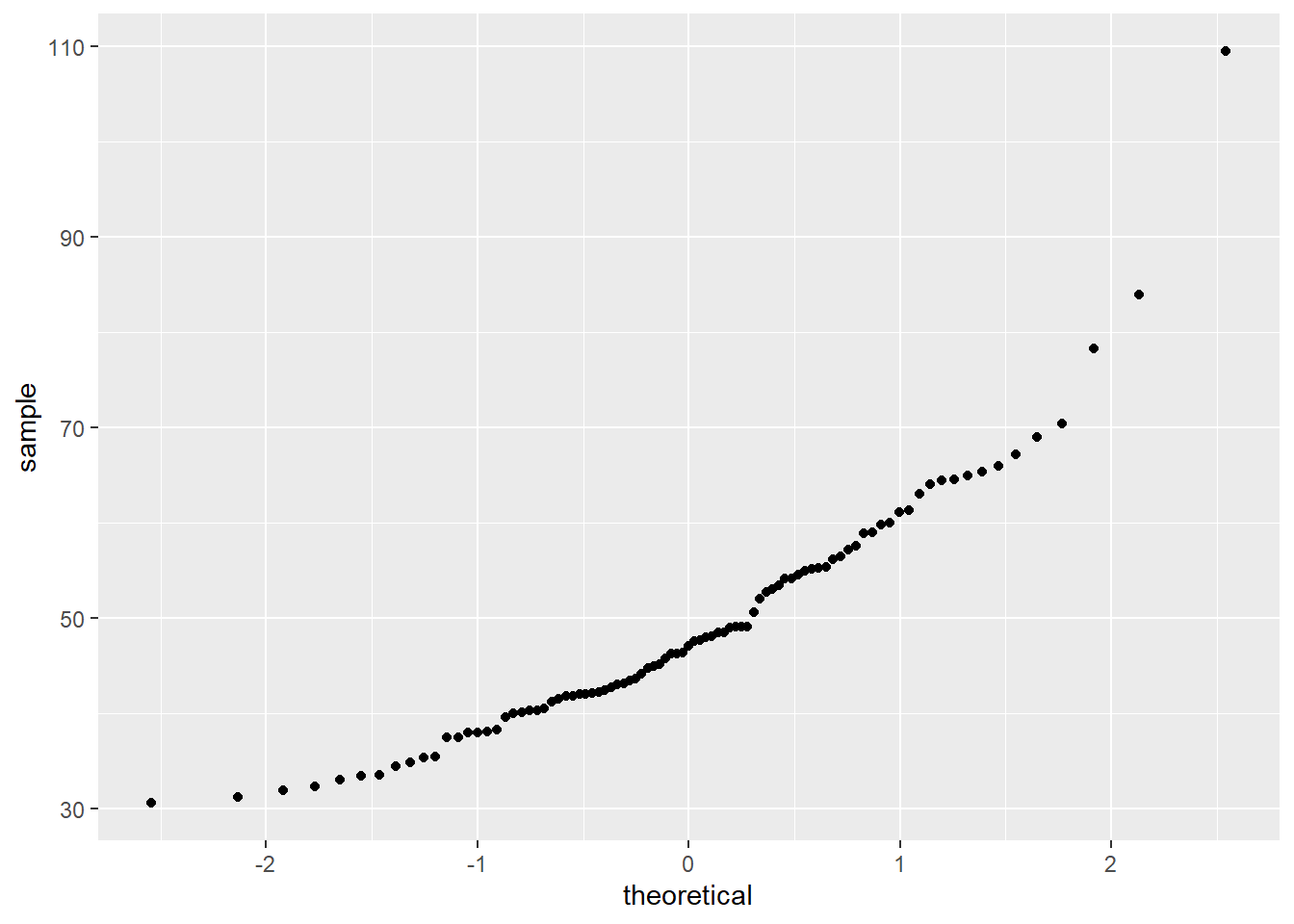
ggplot(dartpoints) + aes(sample = Thickness) + stat_qq()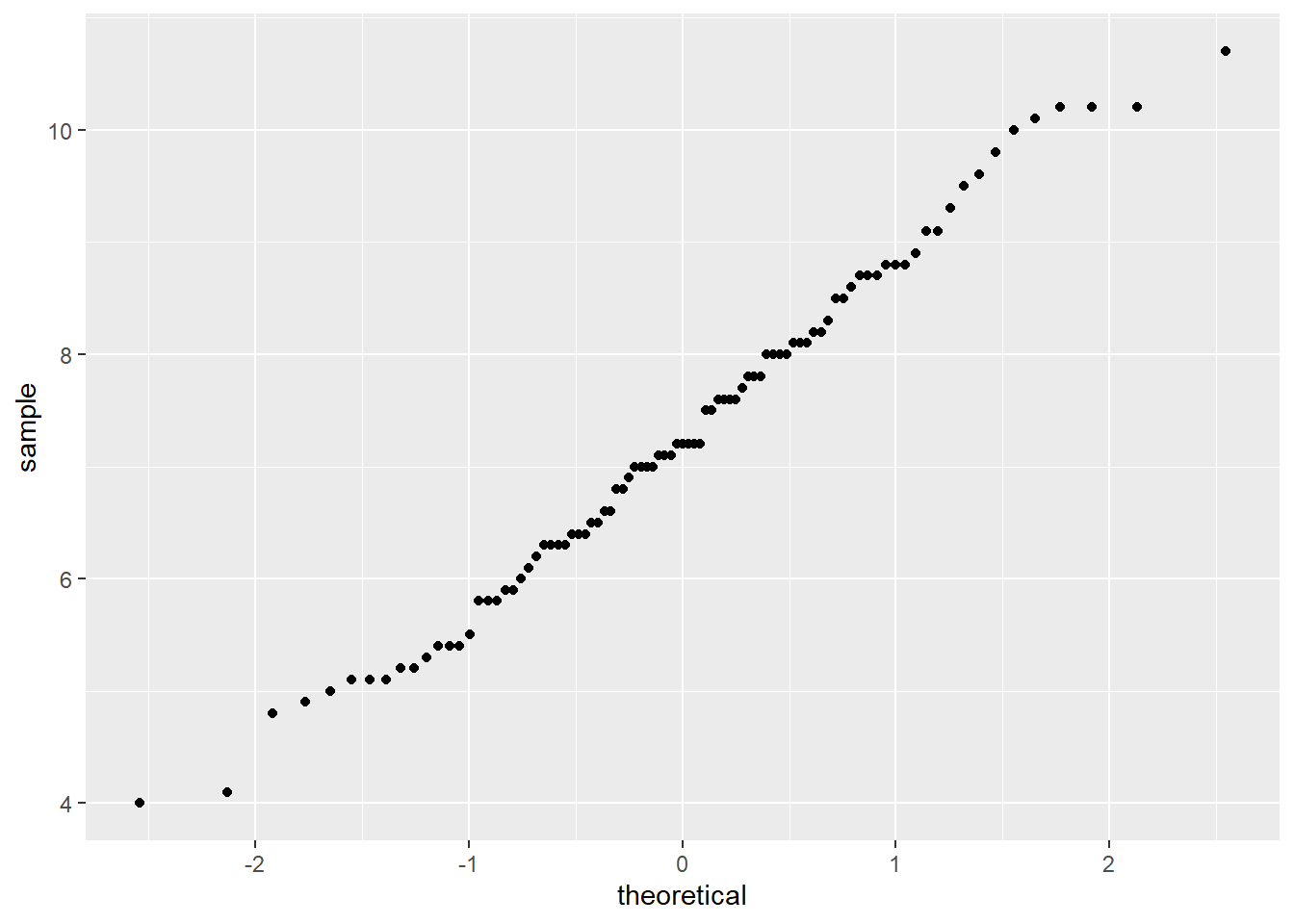
\(H_0\) (null hypothesis): Values fit normal distribution.
\(H_A\) (alternative hypothesis): Values do not fit normal distribution.
p-value: probability of the event that observed values fit normal distribution
p > 0.05: Fail to reject null hypothesis.
Significance level = 0.05 – Event occurs in less than 5% of cases
shapiro.test(dartpoints$Length)
    Shapiro-Wilk normality test

data:  dartpoints$Length
W = 0.90277, p-value = 4.852e-06shapiro.test(dartpoints$Thickness)
    Shapiro-Wilk normality test

data:  dartpoints$Thickness
W = 0.98623, p-value = 0.4559