Considering space

Objectives

Learn what is spatial data.
Learn how spatial data is represented in R.
Learn basic operations with vector data.
Create basic maps.

What is Earth’s shape?

Spheroid
Ellipsoid
Geoid
Potato

Geocentric and local geodetic datums shown on top of a geoid (in false color and the vertical exaggeration by 10,000 scale factor). From Lovelace, Nowosad, Muenchow: Geocomputation with R

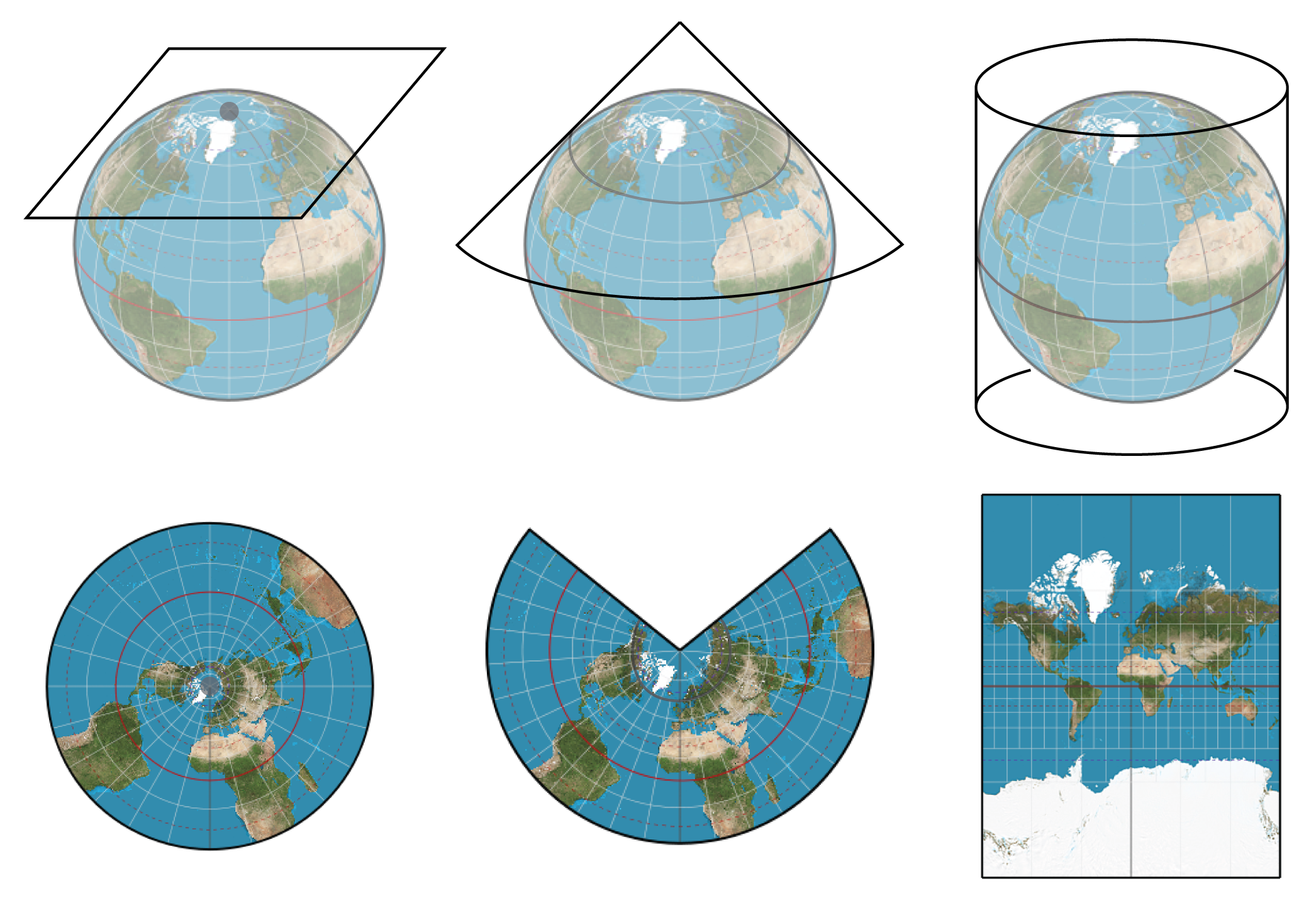
Projections

How to transform a curved surface of an ellipsoid into a plane?

Coordinate reference systems

CRS defines how spatial data relate to the surface of the Earth.

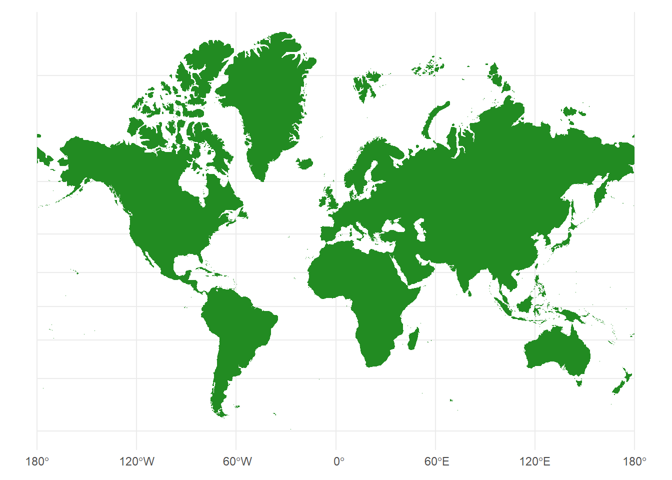
Geographic

WGS 84

EPSG: 4326
latitude: N/S, 0˚ (equator) – 90˚ (poles)
longitude: E/W, 0˚ (prime meridian) – 180° (antimeridian)
in degrees, minutes:
N 49°44.62543', E 15°20.31830'
in decimal degrees:
49.7437572N, 15.3386383E
Package parzer helps to parse coordinates in weird formats.

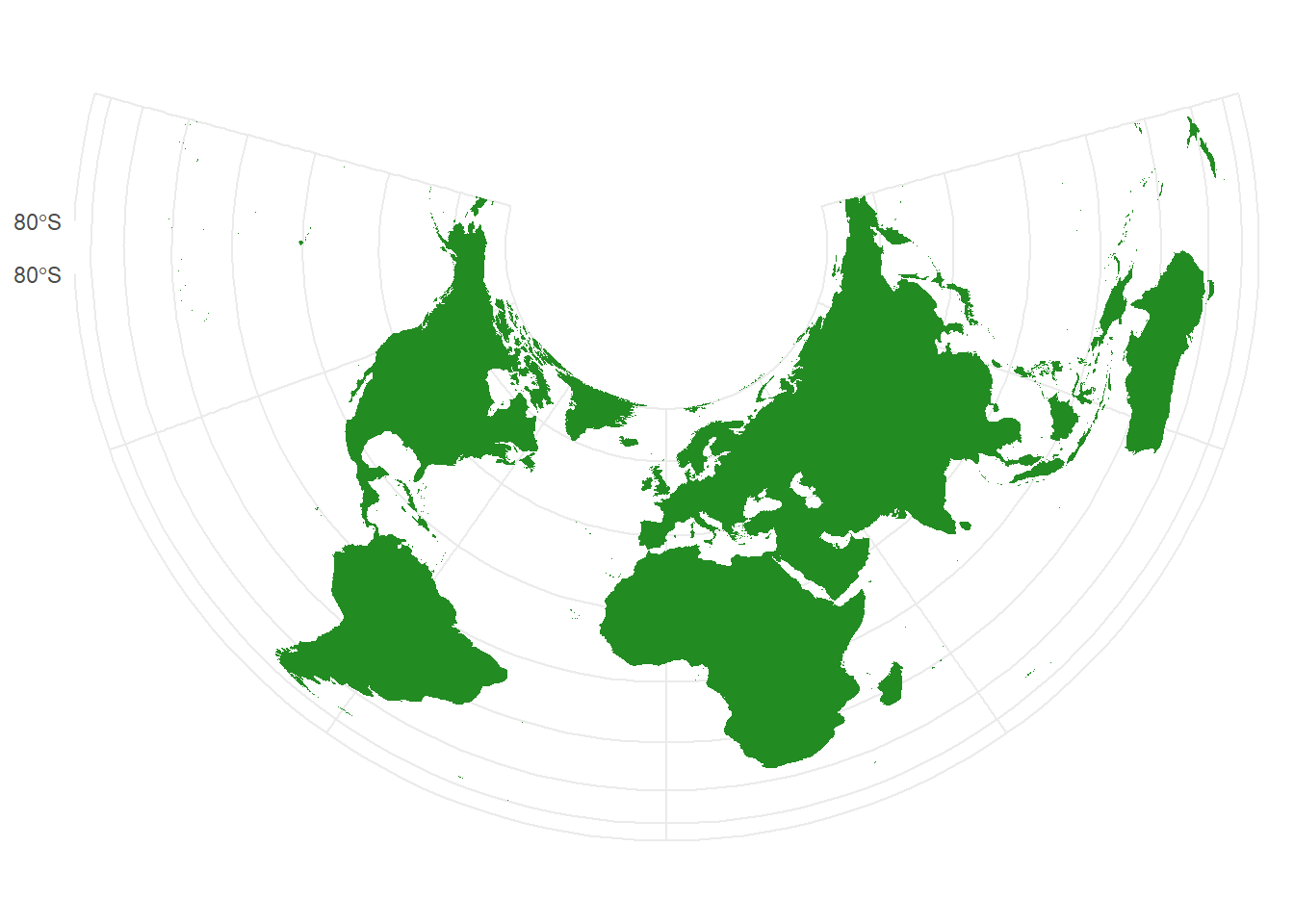
Projected

Many operations can be done only with projected coordinates!

S-JTSK / Křovák East North

EPSG: 5514
Czech Republic and Slovakia
in meters, in negative numbers:
-682473.3, -1089493

WGS 84 / UTM

EPSG for zone 33N: 32633
Czech Republic is in zone UTM 33N

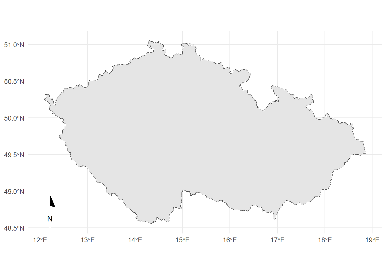
Czech Republic in WGS 84

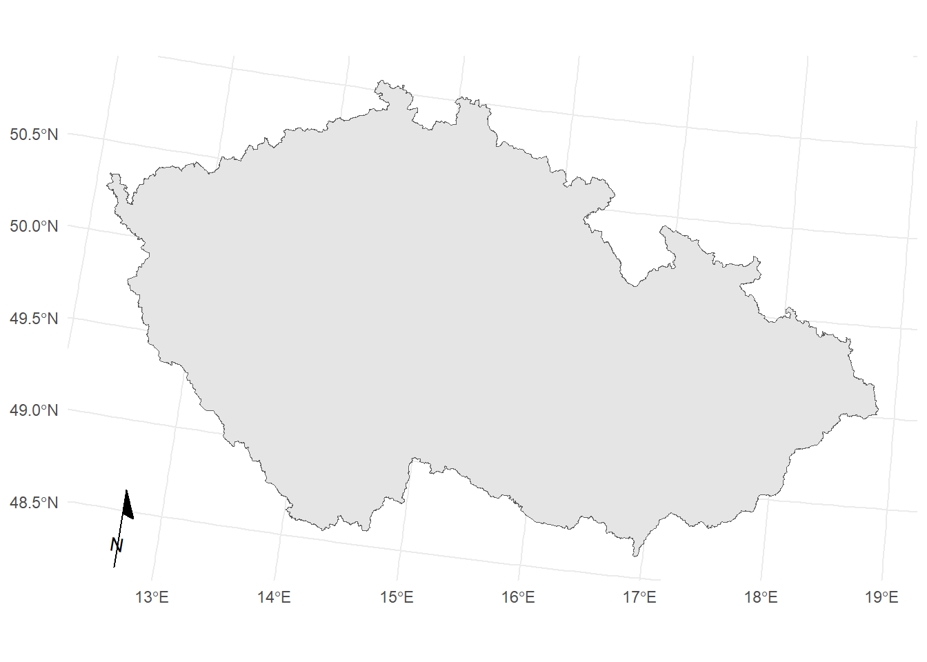
Czech Republic in WGS 84 / UTM

Czech Republic in S-JTSK / Krovak East North

Raster and vector data

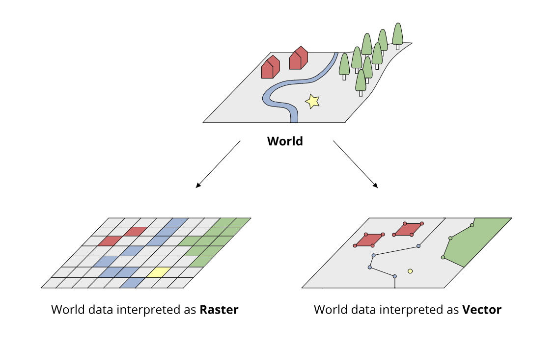
From https://urstudio.sec.sg/wp-content/uploads/2022/03/featured-3.png

Vector data

Points, lines, polygons…

Packages

`sf` package

Vector data, simple features
https://r-spatial.github.io/sf/
Cheatsheet

Raster data

terra package and its predeccessor, raster
stars package – spatiotemporal arrays, raster and vector data cubes

Spatial statistics

spatstat package

Making maps

ggplot2
tmap package – thematic maps
leaflet package – interactive maps

Code along

Dataset

Dataset from Journal of Open Archaeology Data paper
Article DOI: 10.5334/joad.85
Data DOI: 10.5281/zenodo.5728242
Table LASOLES_14C_database.csv

Reading the data

Data is in CSV format, separated by semicolon (;)
Columns Latitude_WGS84 and Longitude_WGS84
Coordinate reference system is WGS 84 (EPSG 4326)

lasoles <- read.csv("./data/LASOLES_14C_database.csv", sep = ";")

# A tibble: 4 × 5
  ID_Date  Latitude_WGS84 Longitude_WGS84 Site_category_ENG Contex_dating_AMCR
  <chr>             <dbl>           <dbl> <chr>             <chr>             
1 CzArch_1           49.1            16.6 hillfort          br.st             
2 CzArch_5           50.1            14.5 settlement        bronz             
3 CzArch_6           49.8            17.0 settlement        ne.lin            
4 CzArch_7           49.8            17.0 settlement        ne.lin

lasoles_wgs84 <- st_as_sf(lasoles, coords = c(x = "Longitude_WGS84", y = "Latitude_WGS84"), crs = 4326)
head(lasoles_wgs84, 4)

Simple feature collection with 4 features and 3 fields
Geometry type: POINT
Dimension:     XY
Bounding box:  xmin: 14.52986 ymin: 49.05189 xmax: 16.95067 ymax: 50.05246
Geodetic CRS:  WGS 84
# A tibble: 4 × 4
  ID_Date  Site_category_ENG Contex_dating_AMCR            geometry
  <chr>    <chr>             <chr>                      <POINT [°]>
1 CzArch_1 hillfort          br.st              (16.62982 49.05189)
2 CzArch_5 settlement        bronz              (14.52986 50.05246)
3 CzArch_6 settlement        ne.lin             (16.95067 49.77669)
4 CzArch_7 settlement        ne.lin             (16.95067 49.77669)

Reprojecting CRS

Function st_transform(x, crs)

EPSG codes:

WGS 84: 4326
S-JTSK East-North: 5514
UTM 33N: 32633
Find more at https://epsg.io/

lasoles_sjtsk <- st_transform(lasoles_wgs84,  crs = "EPSG:5514")
head(lasoles_sjtsk, 4)

Simple feature collection with 4 features and 3 fields
Geometry type: POINT
Dimension:     XY
Bounding box:  xmin: -735634.8 ymin: -1176759 xmax: -566666.7 ymax: -1047924
Projected CRS: S-JTSK / Krovak East North
# A tibble: 4 × 4
  ID_Date  Site_category_ENG Contex_dating_AMCR             geometry
  <chr>    <chr>             <chr>                       <POINT [m]>
1 CzArch_1 hillfort          br.st              (-598287.7 -1176759)
2 CzArch_5 settlement        bronz              (-735634.8 -1047924)
3 CzArch_6 settlement        ne.lin             (-566666.7 -1099048)
4 CzArch_7 settlement        ne.lin             (-566666.7 -1099048)

Making maps

Geom geom_sf()

ggplot(lasoles_sjtsk) +
  geom_sf() +
  theme_minimal()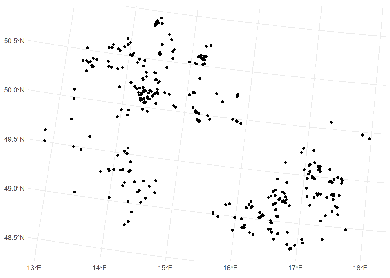

Some background data…

Package RCzechia (Lacko, 2023) has spatial data for the Czech republic…

kraje <- RCzechia::kraje()
head(kraje, 4)

Simple feature collection with 4 features and 3 fields
Geometry type: GEOMETRY
Dimension:     XY
Bounding box:  xmin: 12.40056 ymin: 48.55189 xmax: 15.60422 ymax: 50.61901
Geodetic CRS:  WGS 84
  KOD_KRAJ KOD_CZNUTS3        NAZ_CZNUTS3                       geometry
1     3018       CZ010 Hlavní město Praha MULTIPOLYGON (((14.49806 50...
2     3026       CZ020   Středočeský kraj POLYGON ((15.16973 49.61046...
3     3034       CZ031     Jihočeský kraj MULTIPOLYGON (((15.4962 48....
4     3042       CZ032      Plzeňský kraj MULTIPOLYGON (((13.60536 49...

kraje <- st_transform(kraje, crs = "EPSG:5514")
head(kraje, 4)

Simple feature collection with 4 features and 3 fields
Geometry type: GEOMETRY
Dimension:     XY
Bounding box:  xmin: -891822.3 ymin: -1211576 xmax: -665628.7 ymax: -989063.4
Projected CRS: S-JTSK / Krovak East North
  KOD_KRAJ KOD_CZNUTS3        NAZ_CZNUTS3                       geometry
1     3018       CZ010 Hlavní město Praha MULTIPOLYGON (((-736092 -10...
2     3026       CZ020   Středočeský kraj POLYGON ((-696420.7 -110267...
3     3034       CZ031     Jihočeský kraj MULTIPOLYGON (((-681445.6 -...
4     3042       CZ032      Plzeňský kraj MULTIPOLYGON (((-817386.4 -...

Making maps

ggplot(lasoles_sjtsk) +
  geom_sf(data = kraje) +
  geom_sf() +
  theme_minimal()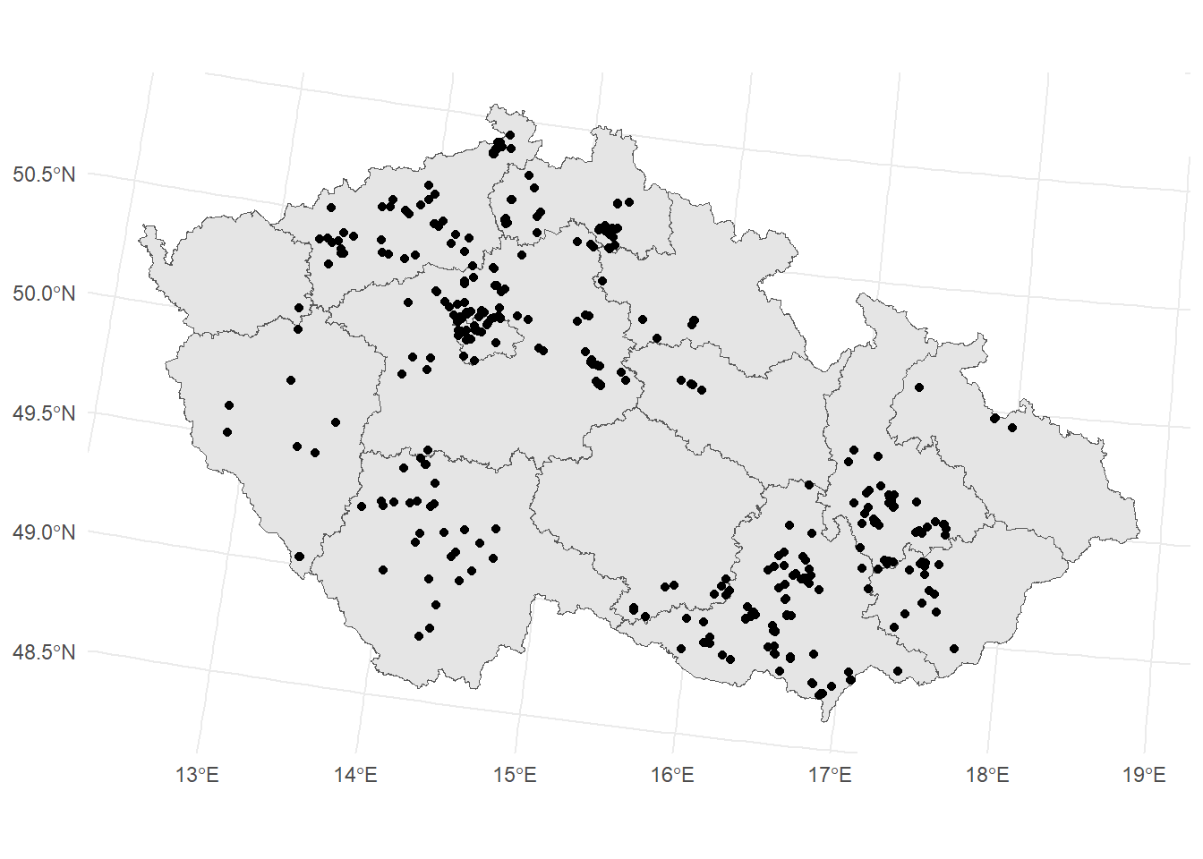

Geometry operations

Unions

st_union()

head(kraje, 2)

Simple feature collection with 2 features and 3 fields
Geometry type: GEOMETRY
Dimension:     XY
Bounding box:  xmin: -816235.3 ymin: -1109600 xmax: -665628.7 ymax: -989063.4
Projected CRS: S-JTSK / Krovak East North
  KOD_KRAJ KOD_CZNUTS3        NAZ_CZNUTS3                       geometry
1     3018       CZ010 Hlavní město Praha MULTIPOLYGON (((-736092 -10...
2     3026       CZ020   Středočeský kraj POLYGON ((-696420.7 -110267...

republika <- st_union(kraje)
republika

Geometry set for 1 feature 
Geometry type: POLYGON
Dimension:     XY
Bounding box:  xmin: -904576.9 ymin: -1227293 xmax: -431722.5 ymax: -935236.5
Projected CRS: S-JTSK / Krovak East North

republika %>% 
  ggplot() +
   geom_sf() +
   theme_minimal()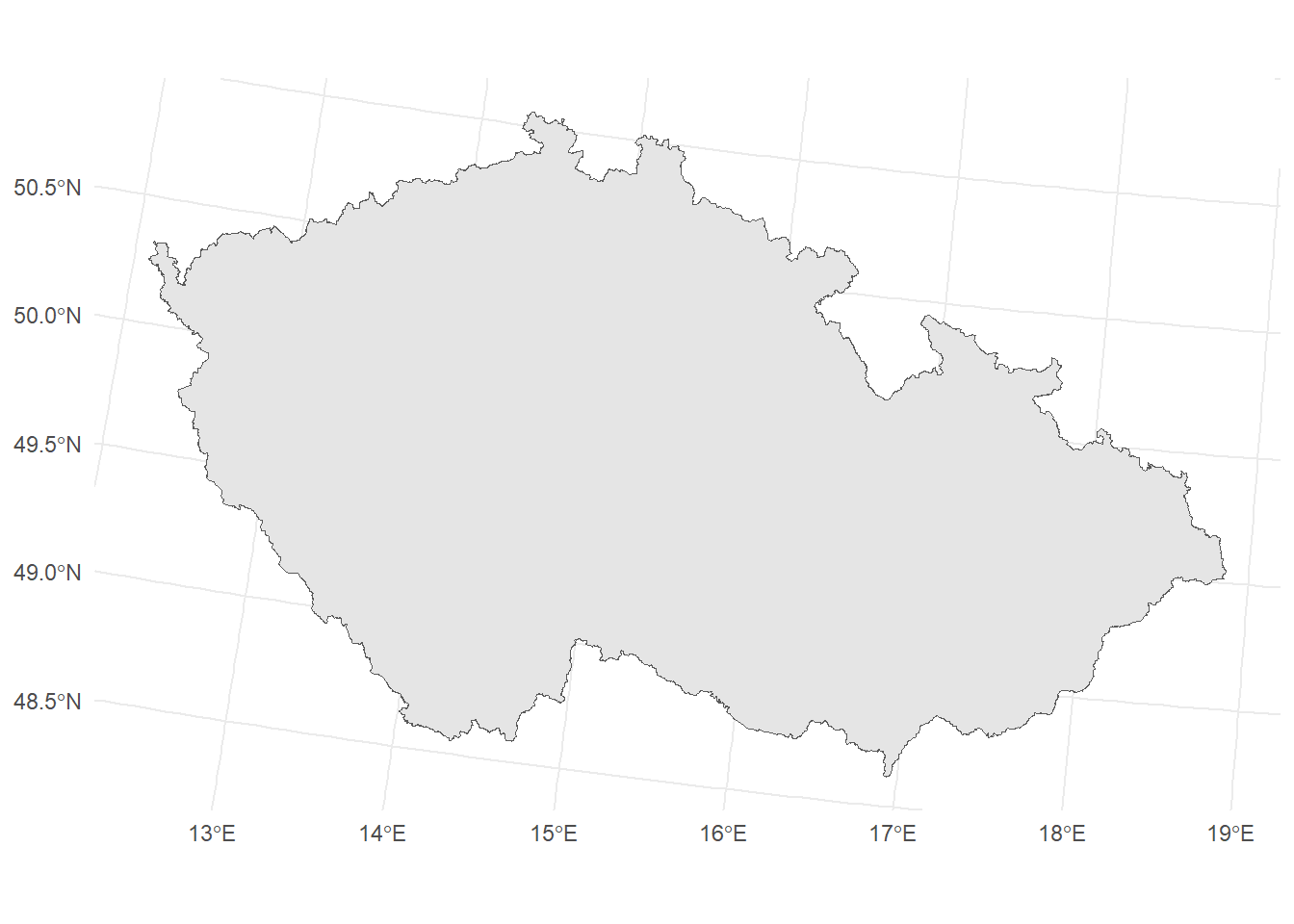

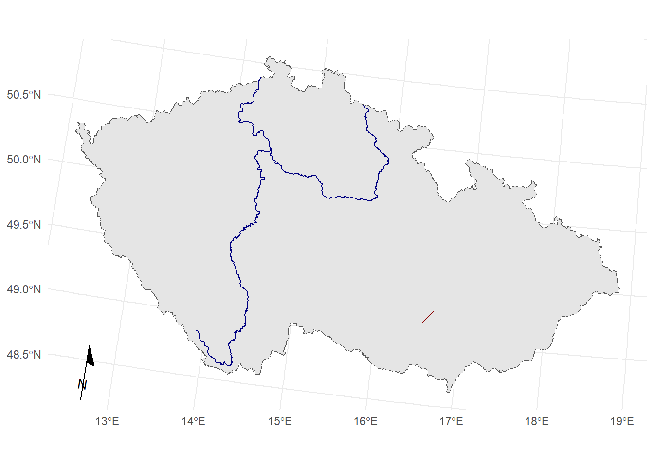
Geometry operations

Centroids

st_centroid()

stred <- st_centroid(republika)
stred

Geometry set for 1 feature 
Geometry type: POINT
Dimension:     XY
Bounding box:  xmin: -682473.1 ymin: -1089493 xmax: -682473.1 ymax: -1089493
Projected CRS: S-JTSK / Krovak East North

ggplot() +
  geom_sf(data = republika) +
  geom_sf(data = stred, size = 4) +
  theme_minimal()

Buffers

st_buffer()

buffer <- st_buffer(stred, 20000)
buffer

Geometry set for 1 feature 
Geometry type: POLYGON
Dimension:     XY
Bounding box:  xmin: -702473.1 ymin: -1109493 xmax: -662473.1 ymax: -1069493
Projected CRS: S-JTSK / Krovak East North

ggplot() +
  geom_sf(data = republika) +
  geom_sf(data = buffer, fill = "forestgreen") +
  geom_sf(data = stred, size = 4) +
  theme_minimal()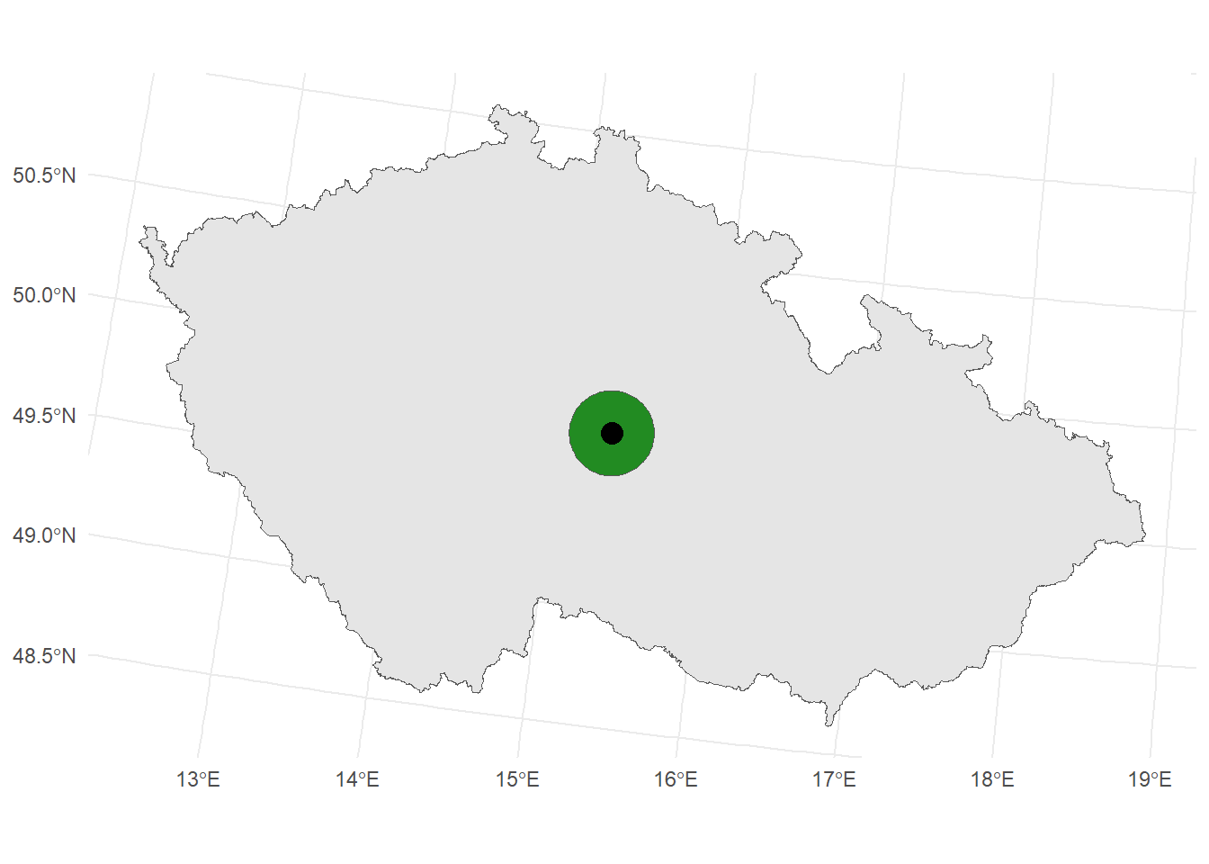

Spatial operations

Topological relations

Many types of raletionships, the most generic one is intersection:
st_intersects(x, y)

prunik <- st_intersects(kraje, stred)
prunik

Sparse geometry binary predicate list of length 14, where the predicate
was `intersects'
first 10 elements:
 1: (empty)
 2: (empty)
 3: (empty)
 4: (empty)
 5: (empty)
 6: (empty)
 7: (empty)
 8: (empty)
 9: (empty)
 10: 1

lengths(prunik)

 [1] 0 0 0 0 0 0 0 0 0 1 0 0 0 0

lengths(prunik) > 0

 [1] FALSE FALSE FALSE FALSE FALSE FALSE FALSE FALSE FALSE  TRUE FALSE FALSE
[13] FALSE FALSE

kraje %>%
  dplyr::filter(lengths(prunik) > 0)

Simple feature collection with 1 feature and 3 fields
Geometry type: MULTIPOLYGON
Dimension:     XY
Bounding box:  xmin: -719989.4 ymin: -1181194 xmax: -607864.3 ymax: -1077931
Projected CRS: S-JTSK / Krovak East North
  KOD_KRAJ KOD_CZNUTS3   NAZ_CZNUTS3                       geometry
1     3107       CZ063 Kraj Vysočina MULTIPOLYGON (((-711377.1 -...

Writing/reading spatial data

st_read() – reads spatial data from the path (data source name, and layer name)
st_write() – writes an object to a specified path (DNS and layer name)

The functions detect what driver to use by the extension.

For vector data, use OGC GeoPackage format (.gpkg)
Do not use ESRI Shapefile (.shp) – it is old and has many limitations (see here for discussion)

st_write(republika, here::here("czrep.gpkg"))

Writing layer `czrep' to data source 
  `<...>/czrep.gpkg' using driver `GPKG'
Writing 1 features with 1 fields and geometry type Polygon.

republika <- st_read(here::here("czrep.gpkg"))

Reading layer `czrep' from data source `<...>/czrep.gpkg' using driver `GPKG'
Simple feature collection with 1 feature and 1 field
Geometry type: POLYGON
Dimension:     XY
Bounding box:  xmin: -904576.9 ymin: -1227293 xmax: -431723.3 ymax: -935236.5
Projected CRS: S-JTSK / Krovak East North

Exercise

Find out how many radiocarbon dated samples are located within distance 15 km (or closer) from Brno.

Brno is this point:

brno <- st_point(c(16.6078411, 49.2002211)) %>% 
          st_geometry() %>% 
          st_set_crs("EPSG:4326")

How many of these radiocarbon dates are from hillforts (Site_category_ENG)?
Create map of the Czech republic with a point showing Brno.
Create a map of all radiocarbon dated samples in Jihomoravský kraj.

Where to learn more…

CRAN Task View: Analysis of Spatial Data
Books:

Objectives

What is Earth’s shape?

Projections

Coordinate reference systems

Geographic

WGS 84

Projected

S-JTSK / Křovák East North

WGS 84 / UTM

Czech Republic in WGS 84

Czech Republic in WGS 84 / UTM

Czech Republic in S-JTSK / Krovak East North

Raster and vector data

Vector data

Packages

sf package

Raster data

Spatial statistics

Making maps

Code along

Dataset

Reading the data

Reprojecting CRS

Making maps

Some background data…

Making maps

Geometry operations

Unions

Geometry operations

Centroids

Buffers

Spatial operations

Topological relations

Writing/reading spatial data

Exercise

Where to learn more…

`sf` package