Relationships

Relationship of quantitative and qualitative variables

Before we continue

Note that there are several ways of how to write qqplot code. Just keep in mind that you always need to specify the data you want to plot, the aesthetic / mapping (aes()) and geometry (geom_) and that you need to separate different layers by + Here are same examples, all are leading to the same result:

ggplot(data = df_dartpoints, mapping = aes(x = Length))+
  geom_histogram()

ggplot(df_dartpoints, aes(x = Length))+
  geom_histogram()

ggplot(df_dartpoints) +
  aes(x = Length) +
  geom_histogram()

plot_1 <- ggplot(df_dartpoints)
plot_1 + aes(x = Length) + geom_histogram()

df_dartpoints %>% ggplot() +
  aes(x = Length) +
  geom_histogram()

NOTE: %>% comes from magrittr package. We will talk about it later

Boxplot

g <- ggplot(df_dartpoints) +
  aes(x = Name, y = Width)

Boxplot

g <- ggplot(df_dartpoints) +
  aes(x = Name, y = Width)
  
g + geom_boxplot()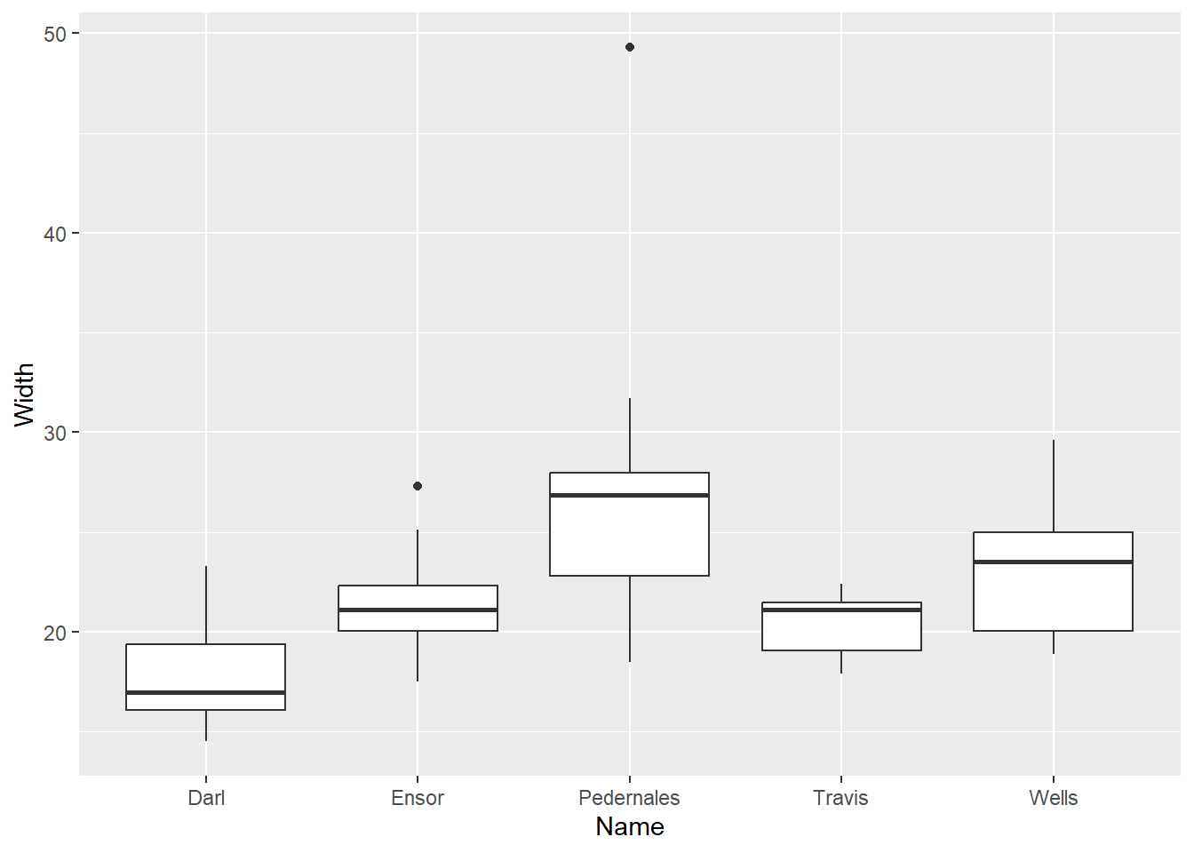

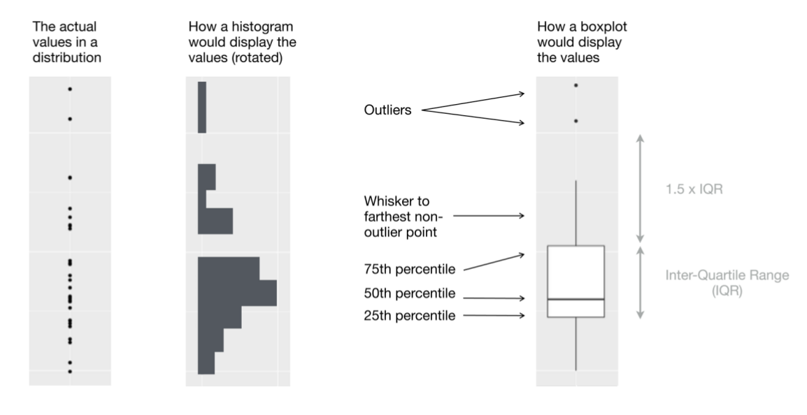
Boxplot

Also box and whisker plot, displays five-number summary.

Violin plot

g + geom_violin()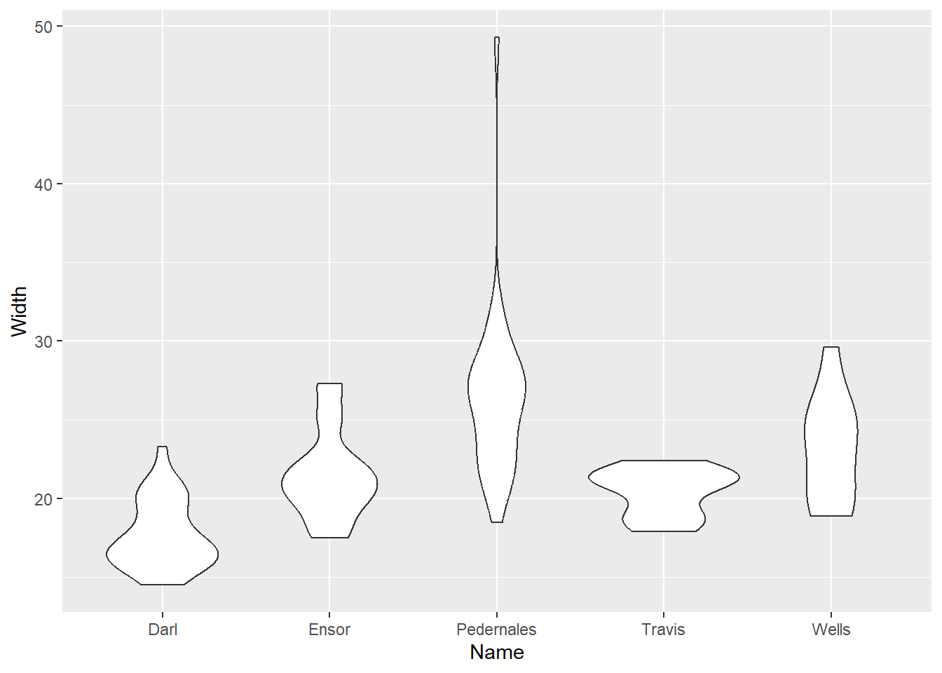

Violin plot

g + geom_violin() +
  geom_jitter(width = 0.05, alpha = 0.4)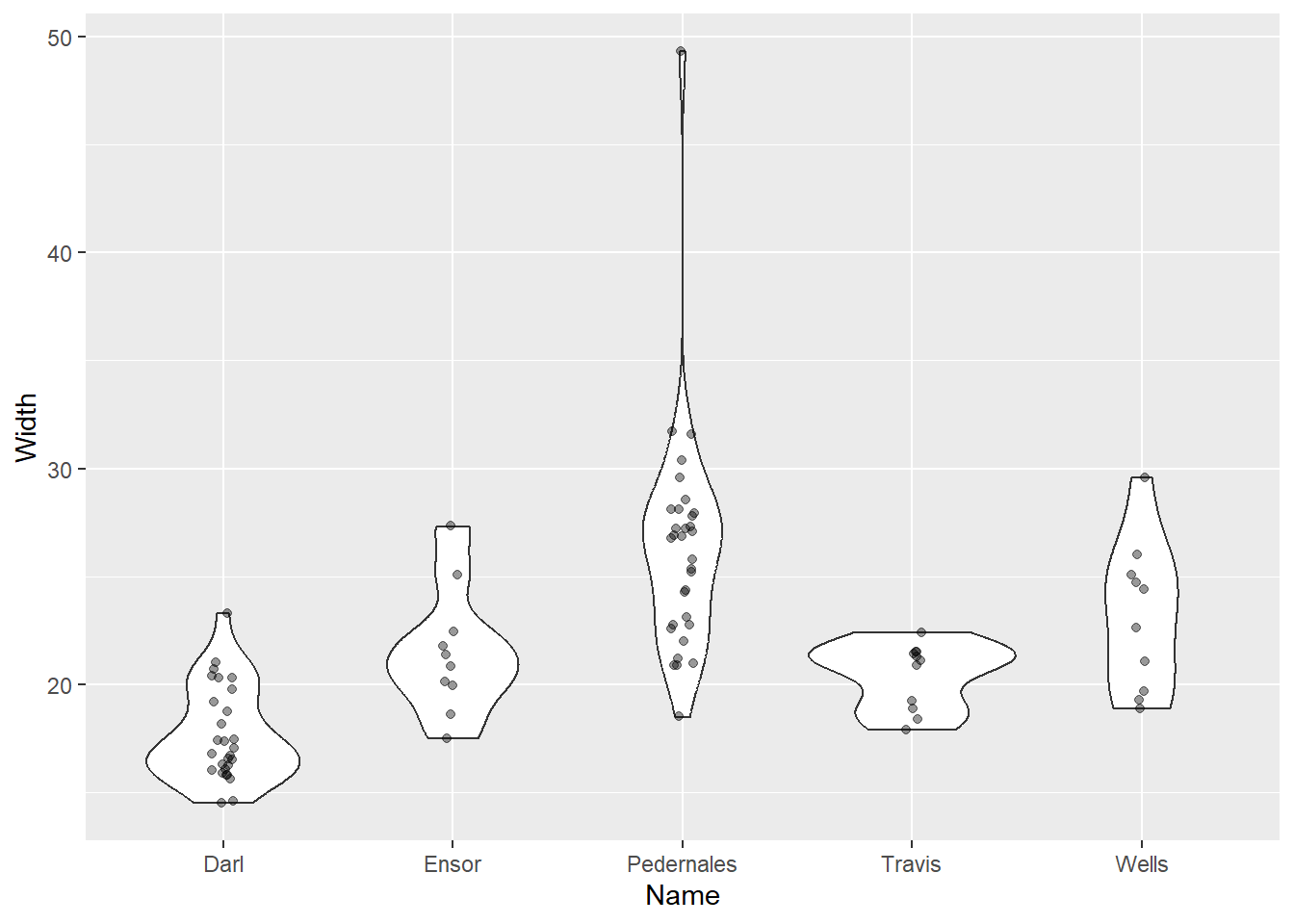

Violin plot

g + geom_violin() +
  geom_boxplot(width = 0.15) +
  geom_jitter(width = 0.05, alpha = 0.2)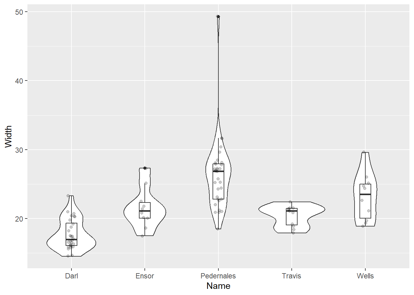

Relationship of two quantitative variables

Correlation

A statistic describing a relationship between two continuous variables.
To what degree is a variable y explained by x?
Correlation coefficient r, from -1 to +1.
Correlation does not imply causation!
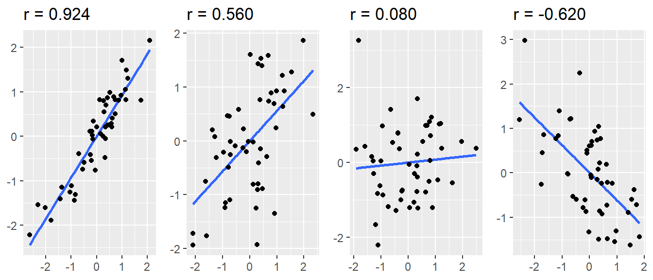
r = 1 – strong positive correlation
r = 0.5 – moderately strong positive correlation
r = 0 – variables are not correlated
r = -0.2 – weak negative correlation
r = -1 – strong negative correlation

Function cor()

cor(df_dartpoints$Length, df_dartpoints$Width)

[1] 0.7689932

cor(df_dartpoints$Length, df_dartpoints$Weight)

[1] 0.879953

cor(df_dartpoints$Width, df_dartpoints$Thickness)

[1] 0.5459291

Scatter plot

Plot displying two continuous variables, x and y.
x axis: explanatory variable, independent, predictor.
y axis: dependent variable, response.

ggplot(df_dartpoints) +
  aes(x = Length, y = Weight) +
  geom_point()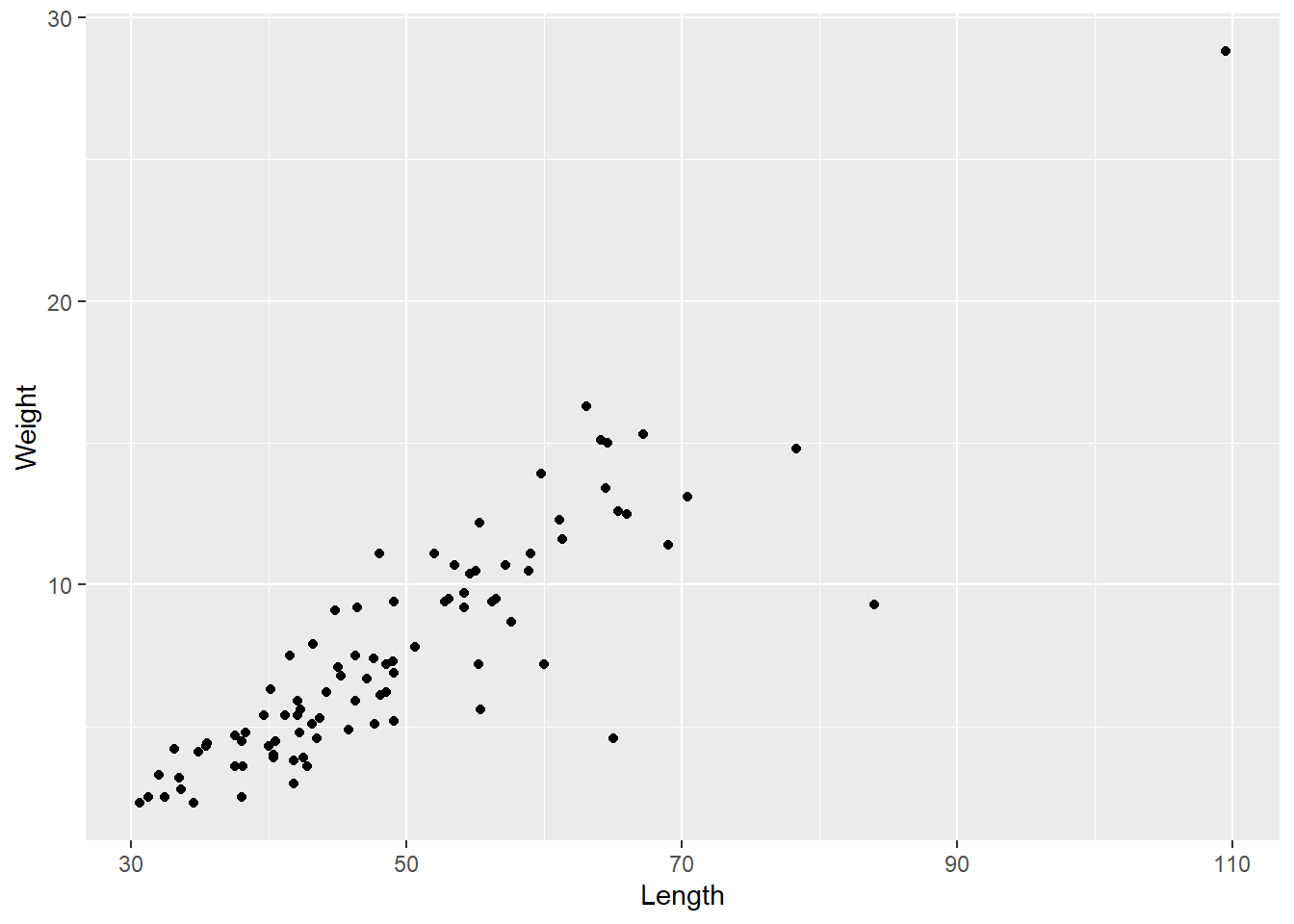

Correlation examples

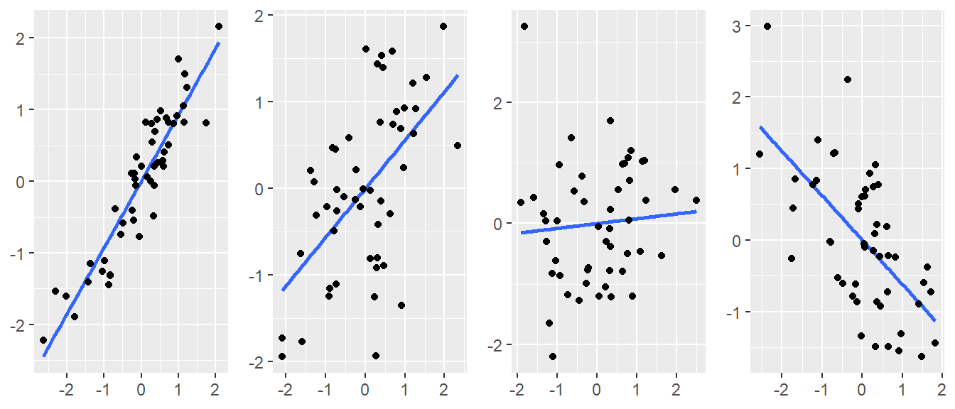
Correlation examples

Scatter plots

We already know scatterplot from the last part:

ggplot(data = df_dartpoints) +
  aes(x = Weight, y = Length) + 
  geom_point(size = 3, alpha = 0.5, color = "steelblue") +
  labs(x = "Weight (g)", y = "Length (mm)",
       title = "Relationship of weight and length of dart points") +
  theme_light()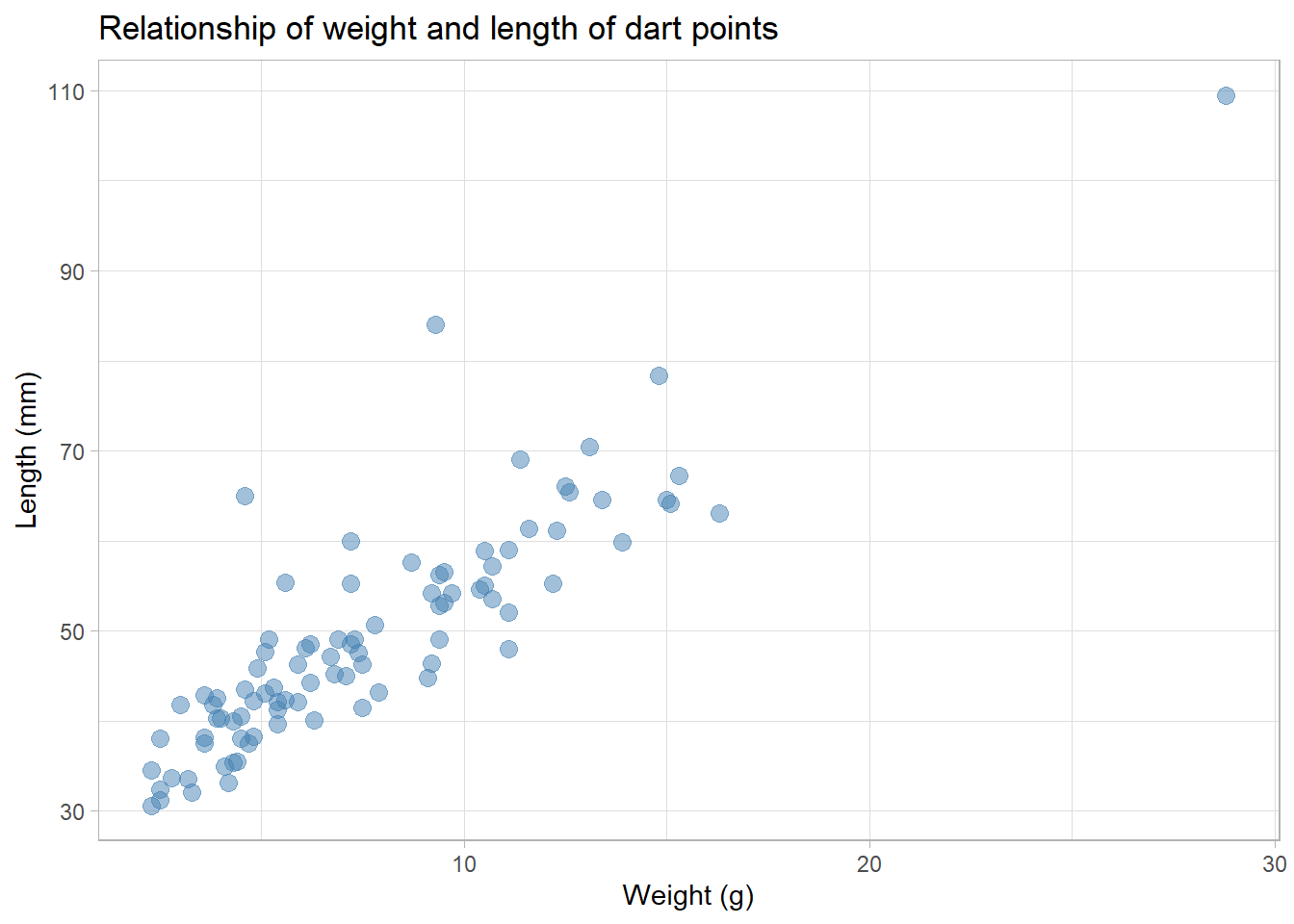

Scatter plots

let’s use geom_smooth() to better see the trend that the points are forming

ggplot(data = df_dartpoints) +
  aes(x = Weight, y = Length) + 
  geom_point(size = 3, alpha = 0.5, color = "steelblue") +
  geom_smooth()+
  labs(x = "Weight (g)", y = "Length (mm)",
       title = "Relationship of weight and length of dart points") +
  theme_light()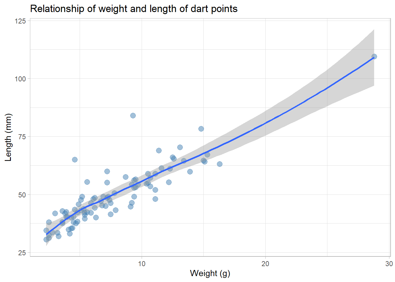

Scatter plots

by method = "lm" you can plot the linear model
se = FALSE will turn off the confidence band

ggplot(data = df_dartpoints) +
  aes(x = Weight, y = Length) + 
  geom_point(size = 3, alpha = 0.5, color = "steelblue") +
  geom_smooth(method = "lm", se = FALSE)+
  labs(x = "Weight (g)", y = "Length (mm)",
       title = "Relationship of weight and length of dart points") +
  theme_light()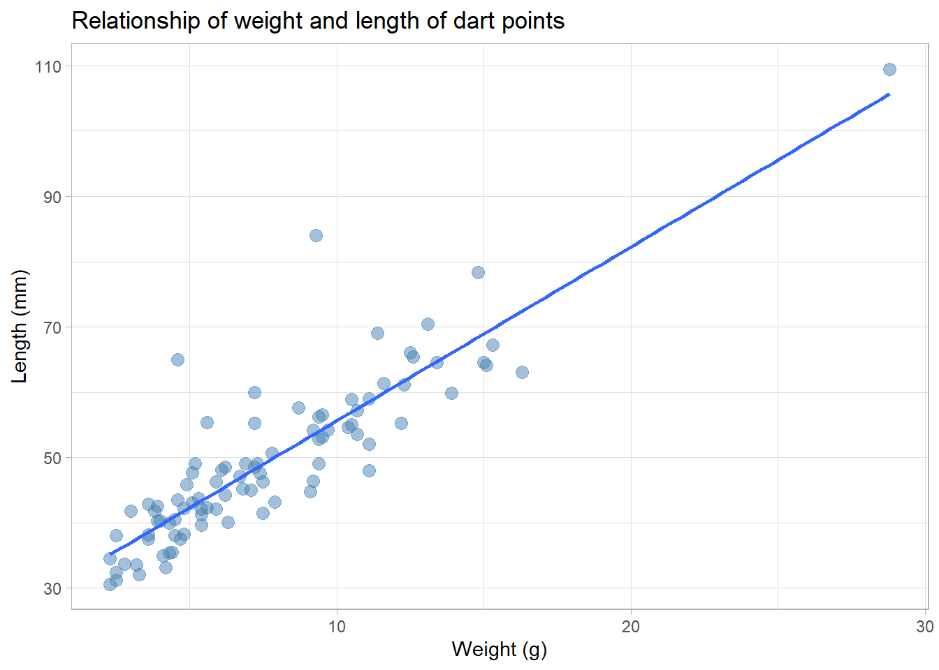

Scatterplots

let’s add another layer and change the theme_:

ggplot(data = df_dartpoints) +
  aes(x = Weight, y = Length) + 
  geom_point(size = 3, alpha = 0.5, color = "steelblue") +
  geom_smooth(method = "lm", se = FALSE)+
  scale_x_continuous(breaks = seq(0, 40, by = 5))+
  scale_y_continuous(breaks = seq(0, 120, by = 10))+
  labs(x = "Weight (g)", y = "Length (mm)",
       title = "Relationship of weight and length of dart points") +
  theme_linedraw()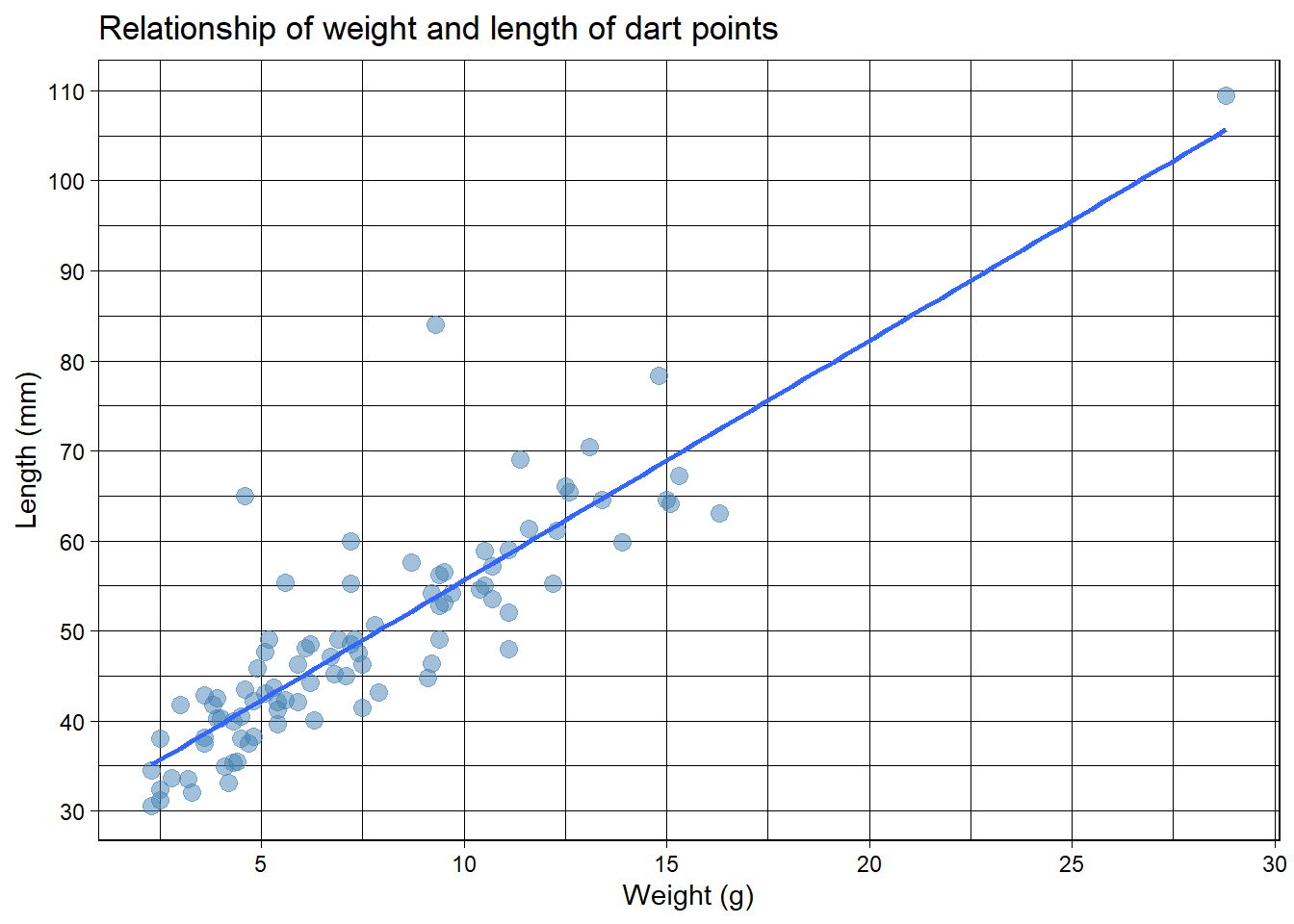

Small multiples

ggplot(data = df_dartpoints) +
  aes(x = Weight, y = Length) + 
  geom_point(size = 3, alpha = 0.5, color = "steelblue") +
  geom_smooth(method = "lm", se = FALSE)+
  scale_x_continuous(breaks = seq(0, 40, by = 5))+
  scale_y_continuous(breaks = seq(0, 120, by = 10))+
  labs(x = "Weight (g)", y = "Length (mm)",
       title = "Relationship of weight and length of dart points") +
  theme_linedraw()+
  facet_wrap(~Name)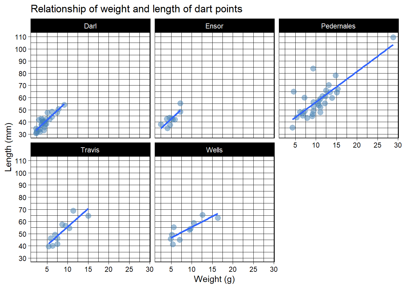

Exercise

Download data set with bronze age cups ( bacups.csv).
Clean your workspace, create a new script and import the data set.
Explore the data set and its structure.
What are the observations?
What types of variables are there?
Create a plot showing distribution of cup heights (H).
Create a boxplot for cup heights divided by phases (Phase).
Are there any outliers?
Count correlation between cup height (H) and rim diameter (RD).
Create a plot showing relationship between cup height and its rim diameter.
Color cups from different phases (Phase) by differently.
Describe the relationship, add a linear model to the plot.
Label the axes sensibly.

Hints:
read.csv(),
str(),
colnames(),
summary(),
cor(),
ggplot() +
aes() +
geom_* + stat_*