Introduction to R
Part 1
Overview
R Basics
1.) Introduction - code along
- orientation in RStudio
- execution command, basic operators
- assigning operator
- vectors
- comments
2.) Syntax and basic functions
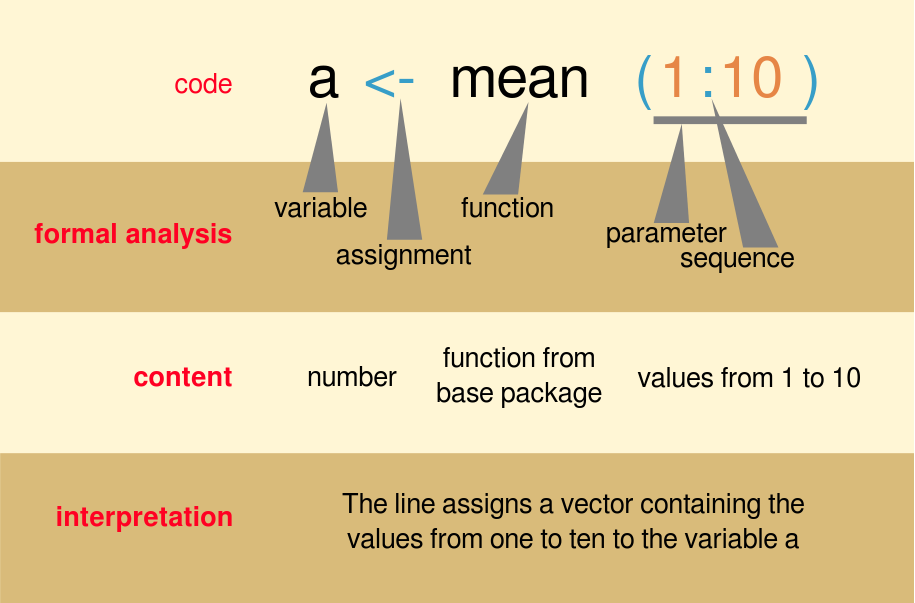
- functions, objects, values, syntax
- dataframes and vectors
Workflow
3.) Workflow
- projects and scripts
- packages
- loading data
Orientation in RStudio
Basic operators
Assigning operator
[1] 10[1] 15[1] 210Creating vectors
Adding comments
Exercise
Task:
1.) create one vector which contains 10 numbers from 51 to 60
2.) and another vector which contains 10 numbers from 101 to 110
3.) save the first vector as “vect_1” and second as “vect_2”
4.) subtract vect_1 from vect_2 and save the results as “vect_sub”
Solution
Functions and syntax
- functions always go with parentheses
() - functions are doing stuff
- syntax:
function_name(argument1 = value1, argument2 = value2, ...)
  [1] 1000 1010 1020 1030 1040 1050 1060 1070 1080 1090 1100 1110 1120 1130 1140
 [16] 1150 1160 1170 1180 1190 1200 1210 1220 1230 1240 1250 1260 1270 1280 1290
 [31] 1300 1310 1320 1330 1340 1350 1360 1370 1380 1390 1400 1410 1420 1430 1440
 [46] 1450 1460 1470 1480 1490 1500 1510 1520 1530 1540 1550 1560 1570 1580 1590
 [61] 1600 1610 1620 1630 1640 1650 1660 1670 1680 1690 1700 1710 1720 1730 1740
 [76] 1750 1760 1770 1780 1790 1800 1810 1820 1830 1840 1850 1860 1870 1880 1890
[91] 1900 1910 1920 1930 1940 1950 1960 1970 1980 1990 2000[1] 101[1] 1000 2000Basic syntax

Objects and values
- there are different types of objects and values in R, each type is allowing you to do different operations
Objects
- for now, it will be enough to introduce vector and dataframe
- vector
- a list of items that are of the same type
- dataframe
- a table
- has rows and columns
- rectangular, ie. identical number of rows in each column.
Values
- similarly, there are many types of values - characters, numbers, factors.
- all you need to know now is that if you want to do mathematic operations, you always have to check whether your numbers are really a numbers and not something else, such as characters
- function
str()will quickly tell you what kind of object with what kind of values you have
Vector
[1] 1 2 3 4 5 6 7 8 9 10 [1] 101 102 103 104 105 106 107 108 109 110 int [1:10] 101 102 103 104 105 106 107 108 109 110 [1] "a" "b" "c" "d" "e" "f" "g" "h" "i" "j" chr [1:10] "a" "b" "c" "d" "e" "f" "g" "h" "i" "j" chr [1:5] "Berlin" "Bratislava" "Prague" "Vienna" "Warsaw"If the vector combines numbers and words, the result will save the numbers as characters, so it is then not possible to make mathematical operations with them
Dataframes
- you can create dataframes by binding the of the same length (!) together
cbind()binds vectors into columns and thenas.data.frame()change them into dataframe
Dataframe - structure
Get the basic information about the dataframe with str()
'data.frame':   10 obs. of  3 variables:
 $ nums : chr  "1" "2" "3" "4" ...
 $ hunds: chr  "101" "102" "103" "104" ...
 $ letts: chr  "a" "b" "c" "d" ...
We see that columns nums and hunds are not numbers, but characters. To be able for us to do mathematic operations, we need to change the values into numbers by function as.numeric()
Subseting data
Square brackets [,]
name_of_your_dataframe[row_number,column_number]
First row
First column
Subseting data with $
Dataframe with atRium participants
Copy, paste and run this whole code chunk:
first_name <- c("Margaux", "Lesley", "Carole", "Alexander", "Dita", "Brigit", "Sara", "Yiu-Kang", "Romane", "Nicky", "Mihailo", "Valeriia", "Carlo", "Panagiotis", "Juan Carlos", "Anna", "Swe Zin", "Ilenia")
country <- c("Lithuania","Ireland","Germany","United Kingdom","Netherlands","Austria","Germany","Germany","Italy","United Kingdom","Serbia","Ukraine","Germany","Italy","France","United Kingdom","Switzerland ","Luxembourg")
position <- c("post_doc","researcher","post_doc","masters_student","post_doc","researcher","phd_student","researcher","phd_student","researcher","researcher","ba_student","post_doc","researcher","researcher","phd_student","phd_student","phd_student")
institution <- c("university","public_research_org","university","university","university","public_research_org","university","public_research_org","university","digital_repository","university","university","public_research_org","public_research_org","private_org","university","university","university")
city <- c("Vilnius","Dublin","Kiel","York","Leiden","Vienna","Kiel","Bochum","Padova","York","Belgrade","Odesa","Leibzig","Rome","Paris","Glasgow","Bern","Luxembourg")
distance_km <- c(850, 1650, 720, 1300, 910, 110, 720, 710, 550, 1300, 560, 1090, 380, 870, 1040, 1590, 720, 760)


df_people <- as.data.frame(cbind(first_name, country, position, institution, city, distance_km))
df_people$distance_km <- as.numeric(df_people$distance_km)
head(df_people, 4)
first_name country position institution city
1 Margaux Lithuania post_doc university Vilnius
2 Lesley Ireland researcher public_research_org Dublin
3 Carole Germany post_doc university Kiel
4 Alexander United Kingdom masters_student university York
distance_km
1 850
2 1650
3 720
4 1300Lets play a bit
What’s your name?
 [1] "Margaux"     "Lesley"      "Carole"      "Alexander"   "Dita"
 [6] "Brigit"      "Sara"        "Yiu-Kang"    "Romane"      "Nicky"
[11] "Mihailo"     "Valeriia"    "Carlo"       "Panagiotis"  "Juan Carlos"
[16] "Anna"        "Swe Zin"     "Ilenia"
Where are you coming from?
 [1] "Lithuania"      "Ireland"        "Germany"        "United Kingdom"
 [5] "Netherlands"    "Austria"        "Italy"          "Serbia"
 [9] "Ukraine"        "France"         "Switzerland "   "Luxembourg"
Which country is most represented?
       Austria         France        Germany        Ireland          Italy
             1              1              4              1              2
     Lithuania     Luxembourg    Netherlands         Serbia   Switzerland
             1              1              1              1              1
       Ukraine United Kingdom
             1              3
Quick Task:
- could calculate which cities are represented?
What is the longest distance one of you had to travel?
Lets play a bit 2
What are your positions?
Who are the PhD students?
   first_name        country    position institution       city distance_km
7        Sara        Germany phd_student  university       Kiel         720
9      Romane          Italy phd_student  university     Padova         550
16       Anna United Kingdom phd_student  university    Glasgow        1590
17    Swe Zin   Switzerland  phd_student  university       Bern         720
18     Ilenia     Luxembourg phd_student  university Luxembourg         760
Alternative - selecting specific columns
   first_name    position       city
7        Sara phd_student       Kiel
9      Romane phd_student     Padova
16       Anna phd_student    Glasgow
17    Swe Zin phd_student       Bern
18     Ilenia phd_student Luxembourg
Quick Task:
- can you subset row with your name and check whether I didn’t messed up your data?
Exercise
Task:
Use the dataframe df_people to solve this questions:
- What are the names of the variables in the dataframe?
- Which types of institution are represented here?
- Which types of institution are most represented here?
- What is the average distance between Brno and the cities?
- Who are the postdocs and from which cities are they coming?
Hints: names(), unique(), table(), mean(),[,]
Solution
- What are the names of the variables in the dataframe?
Alternative:
- Which types of institution are represented here?
[1] "university"          "public_research_org" "digital_repository"
[4] "private_org" - Which types of institution are most represented here?
Solution
- What is the average distance between Brno and the cities?
Alternative
   Min. 1st Qu.  Median    Mean 3rd Qu.    Max.
110.0 712.5 805.0 879.4 1077.5 1650.0 - Who are the postdocs and what distance did they have to travel?
Other useful functions for dataframe
str()- reveals the structure of the dataframe
'data.frame':   18 obs. of  6 variables:
 $ first_name : chr  "Margaux" "Lesley" "Carole" "Alexander" ...
 $ country    : chr  "Lithuania" "Ireland" "Germany" "United Kingdom" ...
 $ position   : chr  "post_doc" "researcher" "post_doc" "masters_student" ...
 $ institution: chr  "university" "public_research_org" "university" "university" ...
 $ city       : chr  "Vilnius" "Dublin" "Kiel" "York" ...
$ distance_km: num 850 1650 720 1300 910 110 720 710 550 1300 ...head(),tail()
  first_name   country   position         institution    city distance_km
1    Margaux Lithuania   post_doc          university Vilnius         850
2 Lesley Ireland researcher public_research_org Dublin 1650 first_name country position institution city distance_km
17 Swe Zin Switzerland phd_student university Bern 720
18 Ilenia Luxembourg phd_student university Luxembourg 760ncol(),nrows(),
sum()
Workflow
- scripts
- projects
- packages
- loading data
Scripts
# Practice script for atRium training school 2024
# Author: Peter Tkáč
# Date: 2024-09-10

## ---- Packages
library(here)
library(tidyverse)

## ---- Data Loading

df_darts <- read.csv(here("data/dartpoints.csv"))
str(df_darts)

## ---- Basic summaries

nrow(df_darts) # number of dartpoints
table(df_darts$Name) # numer of types of the dartpoints

## ---- Plots

ggplot(df_darts, aes(x=Name))+
  geom_bar(fill = "pink")+
  theme_light()

## ---- Saving result

ggsave(filename = "very_important_plot.png")
Projects
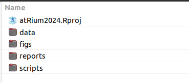
.Rprojfile - a “storage” of your scripts, data…- we recommend you to use parent folder to store your project file and then sub-folders to store data, figures, scripts, etc.

Packages
- by installing additional packages, you can expand the amount of things you can do in R
- there are plenty of packages with different functions and aims
- basic principle will be introduced by package “here”
#install.packages("here") # installs the package
library(here) # loads the package
here() # runs a function from the package
[1] "C:/Users/pajdla/Documents/projects/atRium"you only need to install the package once
install.packages("name_of_the_package"), but it needs to be loaded every time you start a new script or after you have cleaned up your workspacelibrary(name_of_the_package)sometime you need to specify from which package your function is:
name-of-the-package::name-of-the-function()
  first_name country    position institution city distance_km
1     Carole Germany    post_doc  university Kiel         720
2       Sara Germany phd_student  university Kiel         720
If you are not sure from which package your function is coming, you can easily find out by:
Loading data
- download data dartpoints.csv and move them to your project file
Paths
Absolute file path - The file path is specific to a given user.
C:/Documents/MyProject/data/dartpoints.csv
Relative file path If I am currently in MyProject/ folder:
./data/dartpoints.csv
Package here()
- Package
hereis here to save the day! - Function
here()will know where the top directory is, so you do not need to write whole URL adress
Try running here() to see where your project is stored
Loading data
An example of loading data with here() function:
- NOTE that in this case data which you want to load have to be in a subfolder “data” which is located in the same folder as your project
read.csvloads .csv files (AKA comma-separated values file) into your R- if the values in your file are separated by other way, you have to adjust. For example for values separated by semicolom
;use argumentsep=";":
Exercise
Observe the dartpoint data
- How many observations and how many variables are in the dataframe?
- What are the names of the variables?
- Are there any quantitative variables? Are they stored properly as numbers so we can make mathematic operations?
- What is the mean length of the dartpoints?

atRium training school, Brno 2024 | Intro to R