Introduction to R
Part 2
Visualising your data with packgage ggplot2
Inspiration

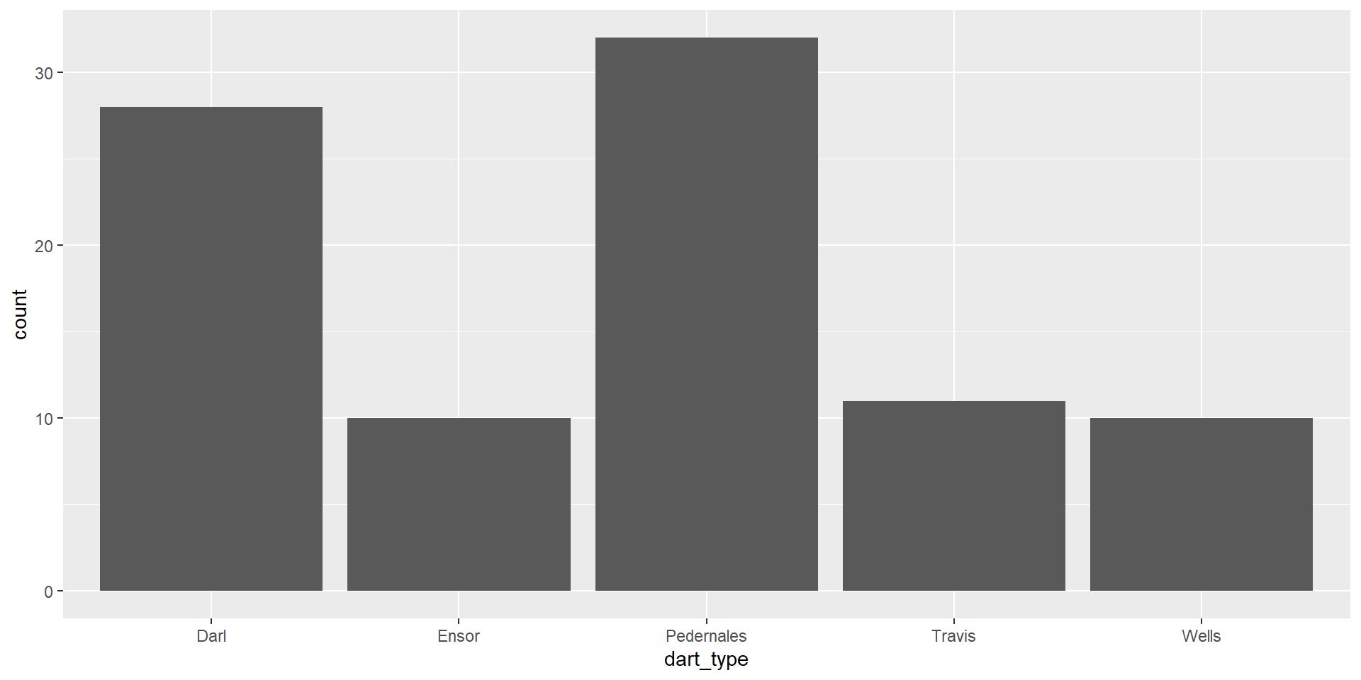
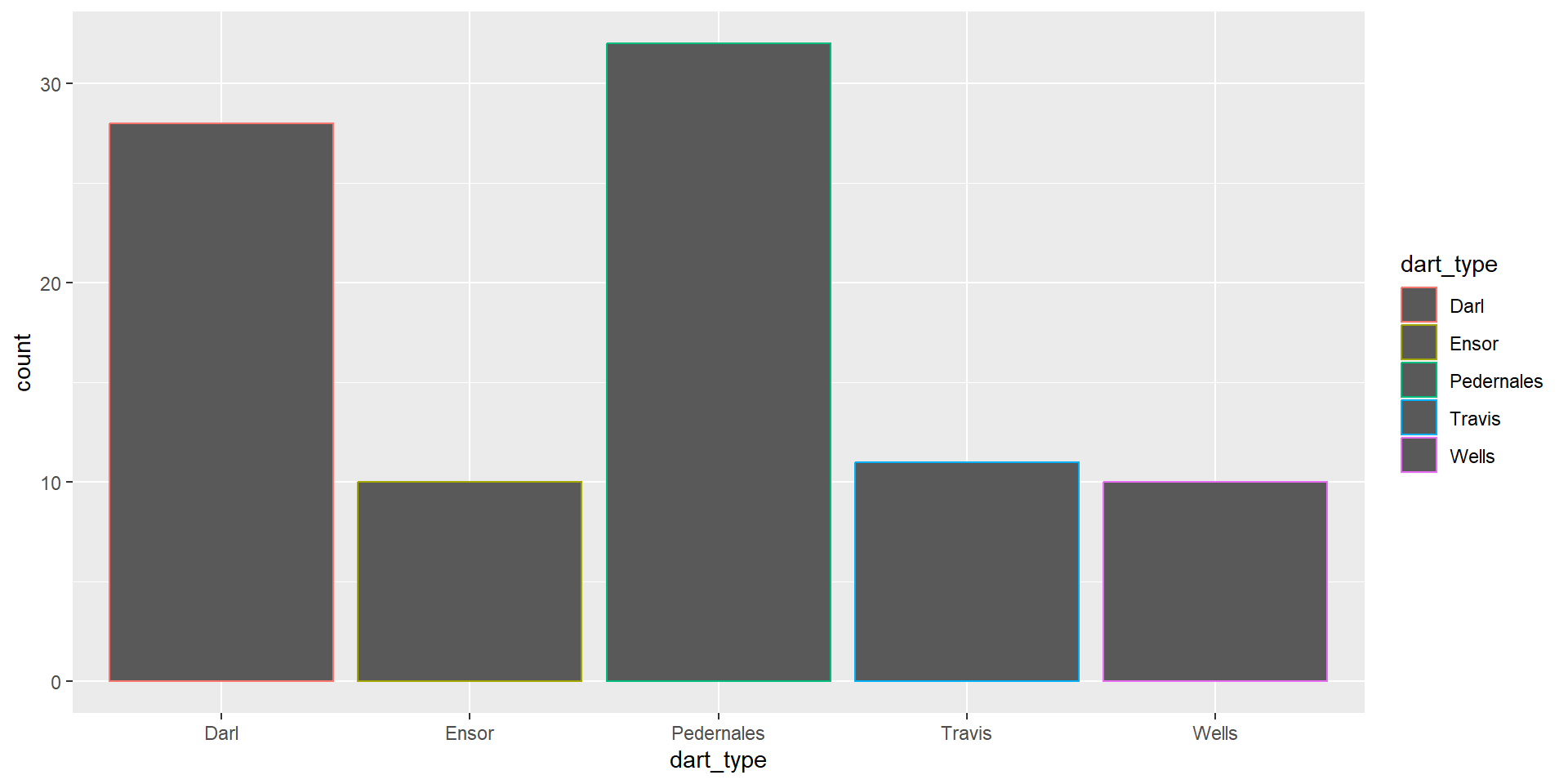
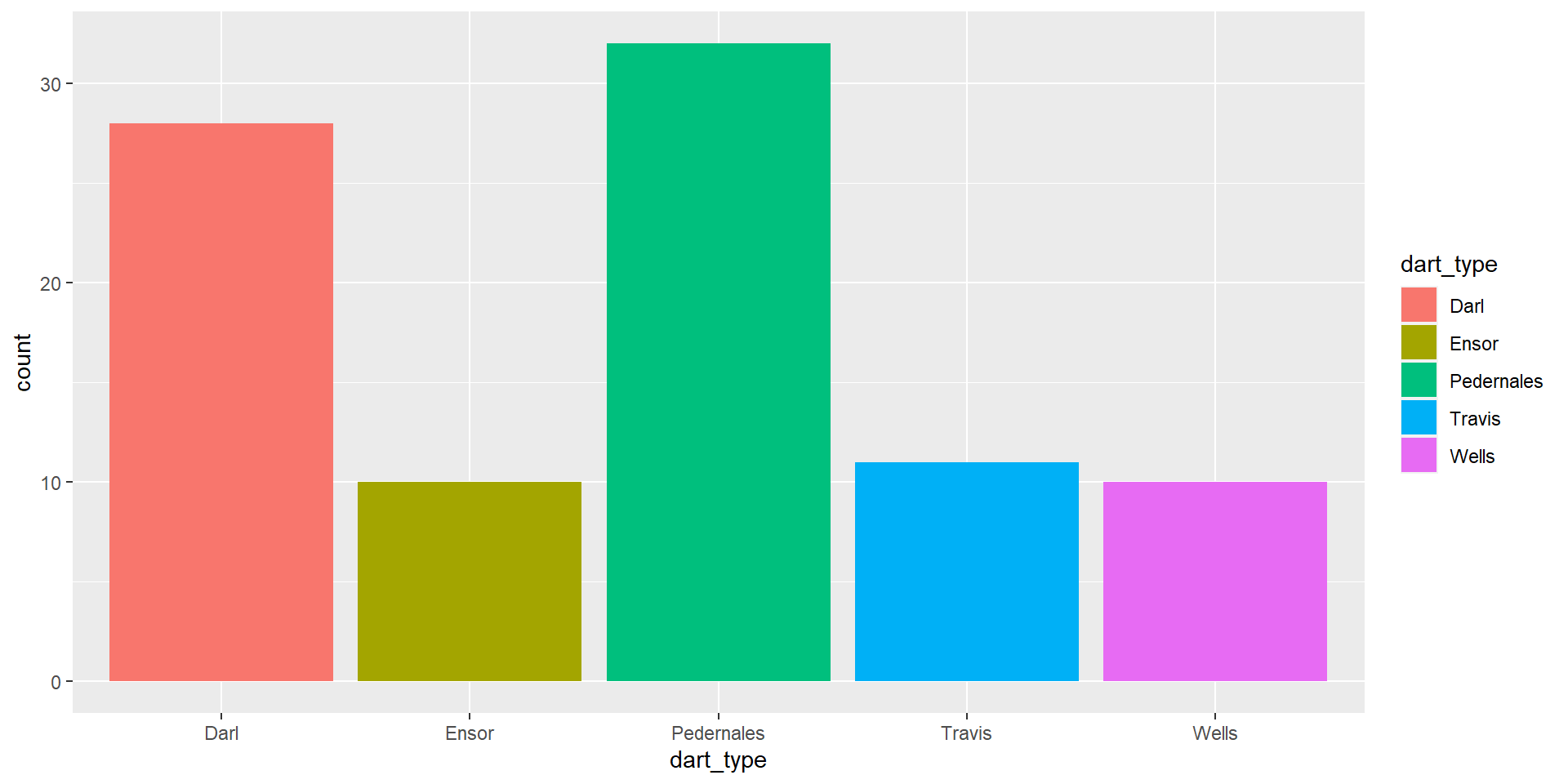
Basic types of ggplot - barplot
- for one variable
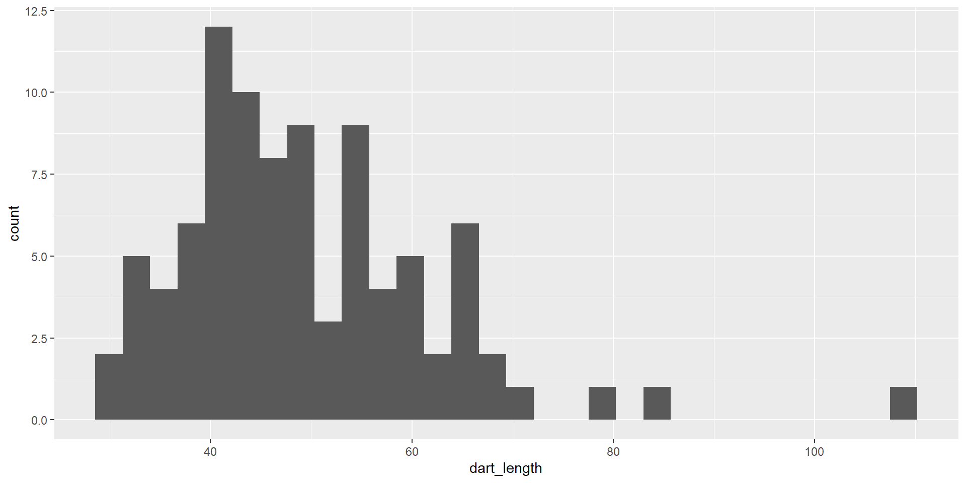
Basic types of ggplot - histogram
- distribution of one variable
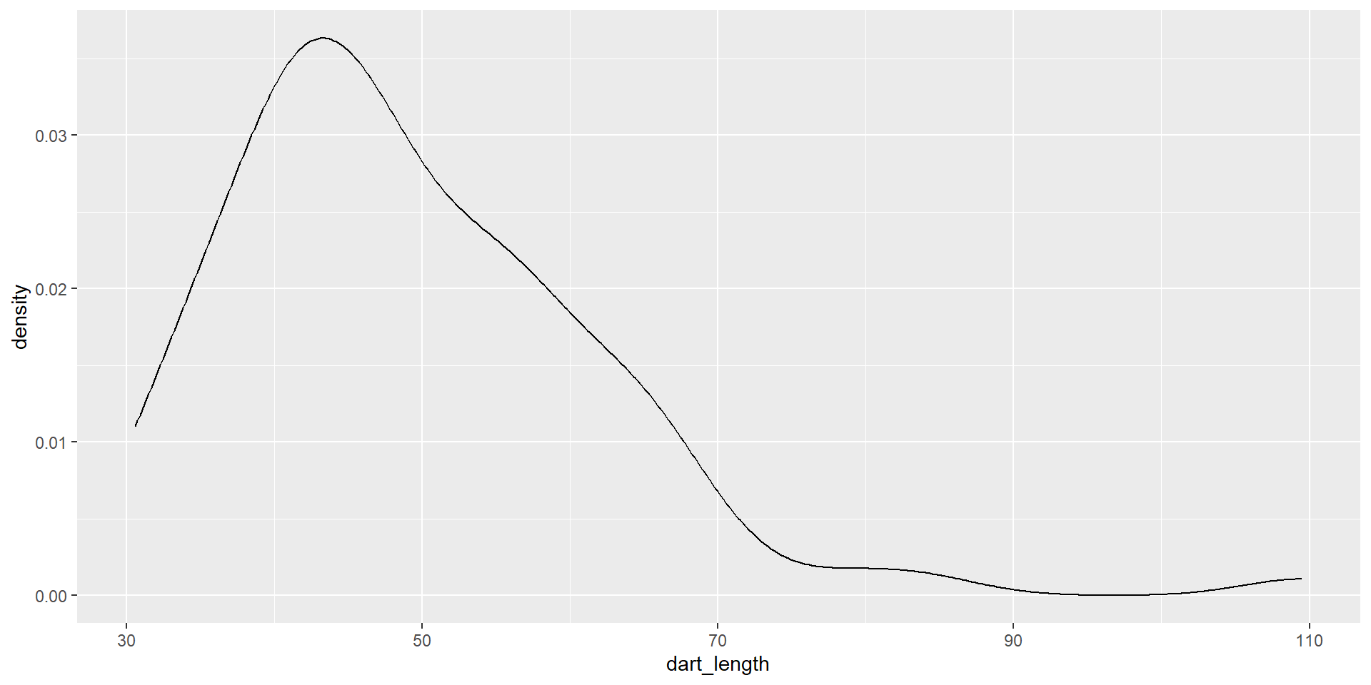
Basic types of ggplot - density plot
- distribution of one variable

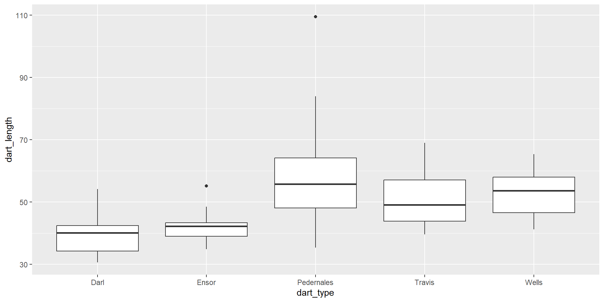
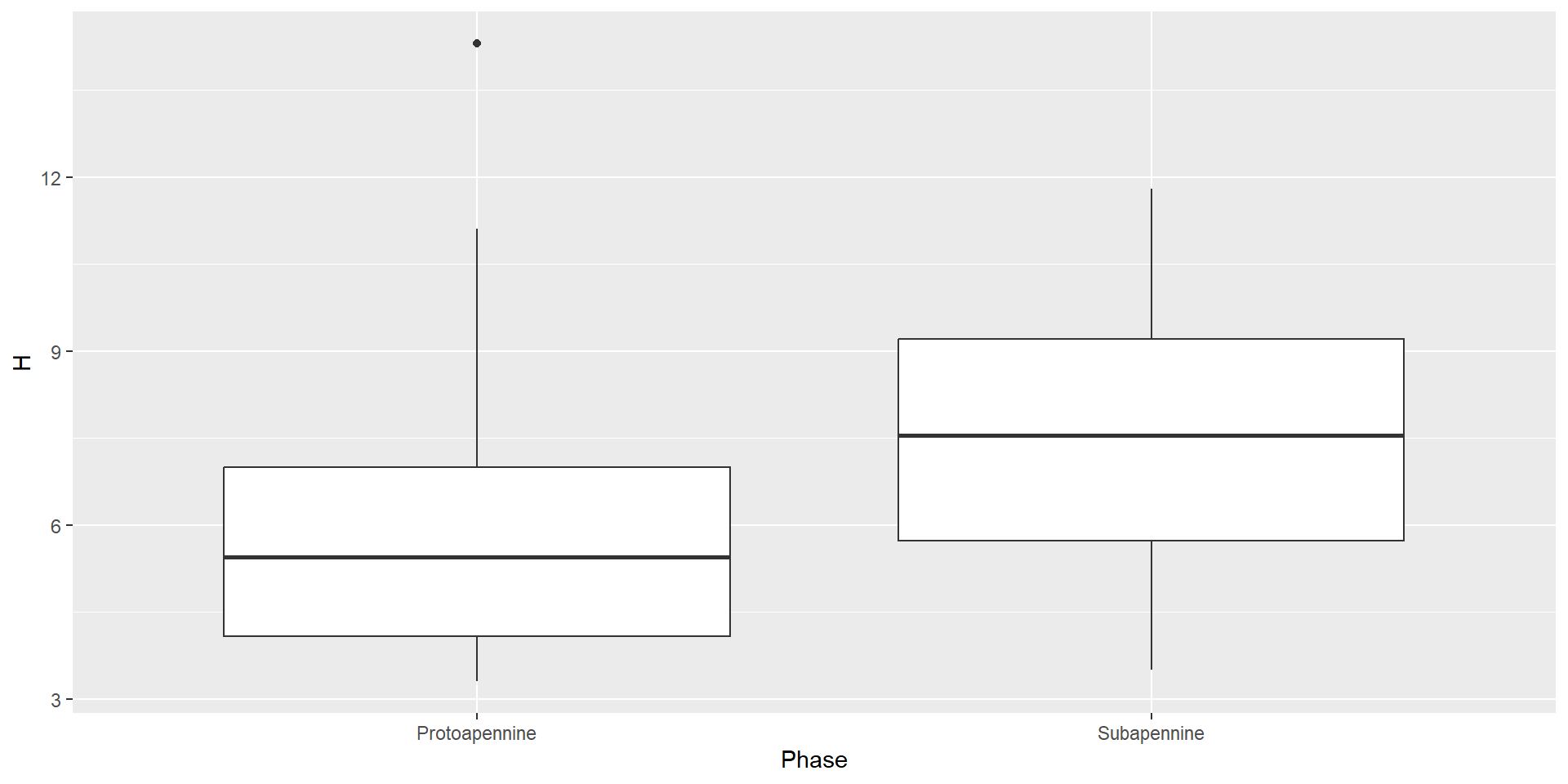
Basic types of ggplot - boxplot
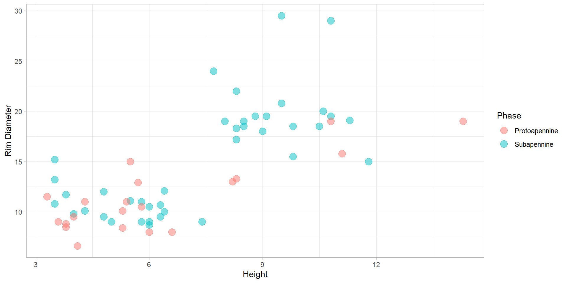
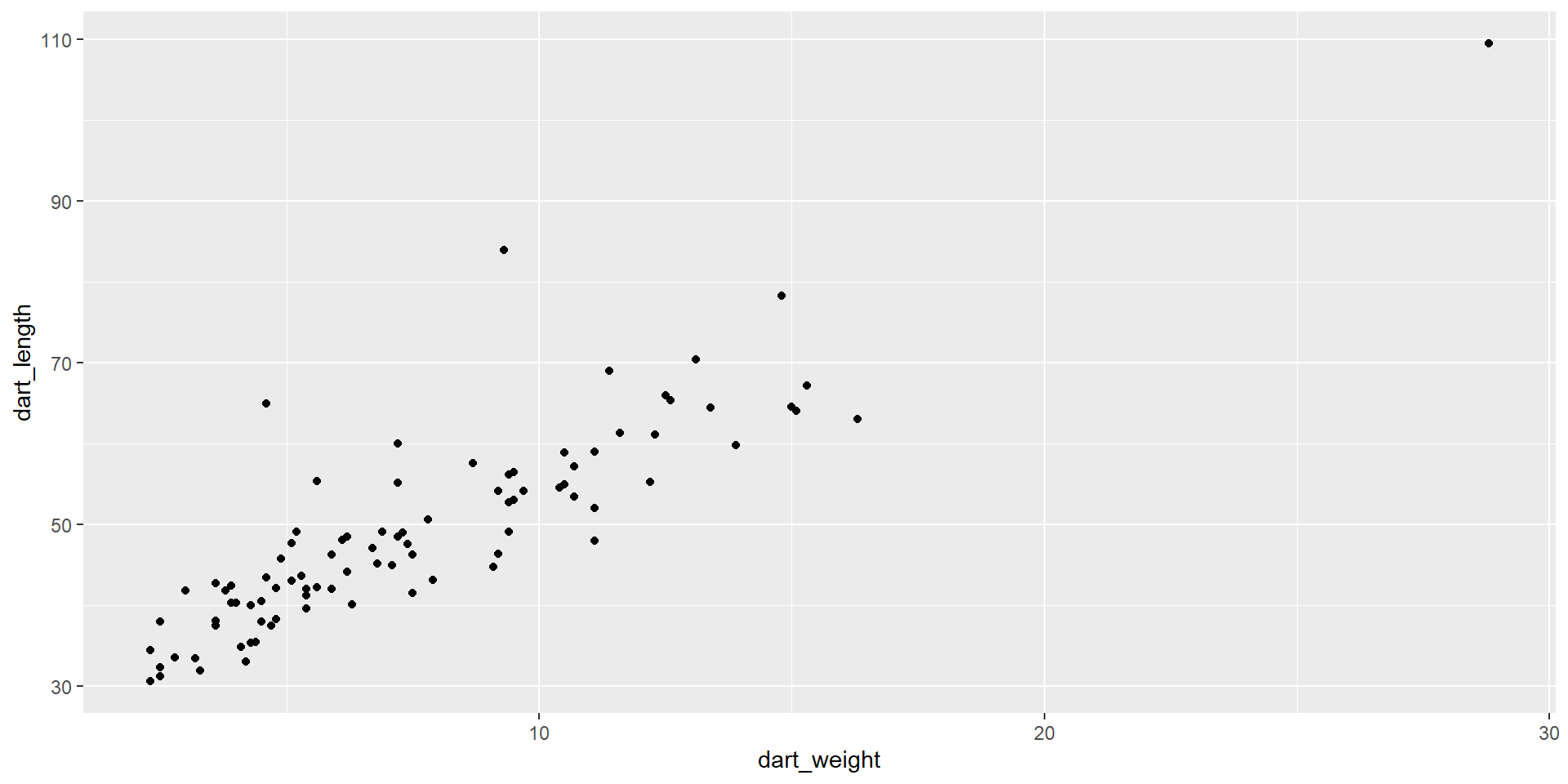
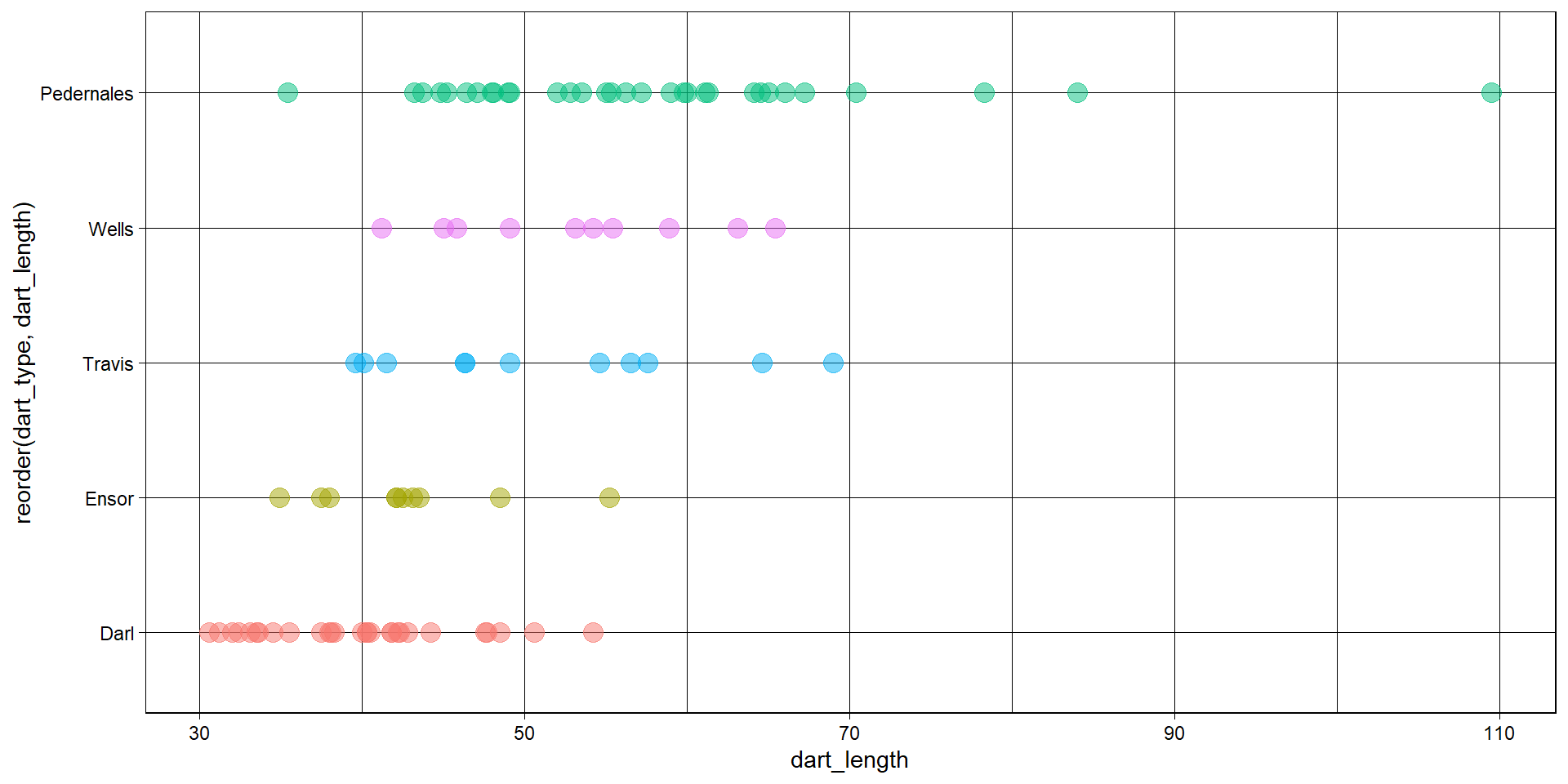
Basic types of ggplot - scatter plot
- comparing two or more variables
Refining your plot
Lets go back to the scatterplot and play a little
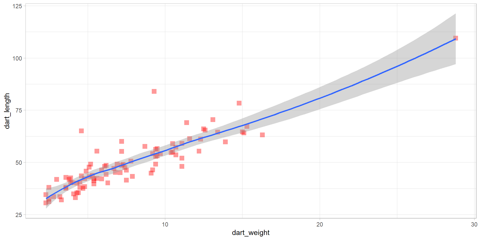
Task:
- try different colours, shapes and themes
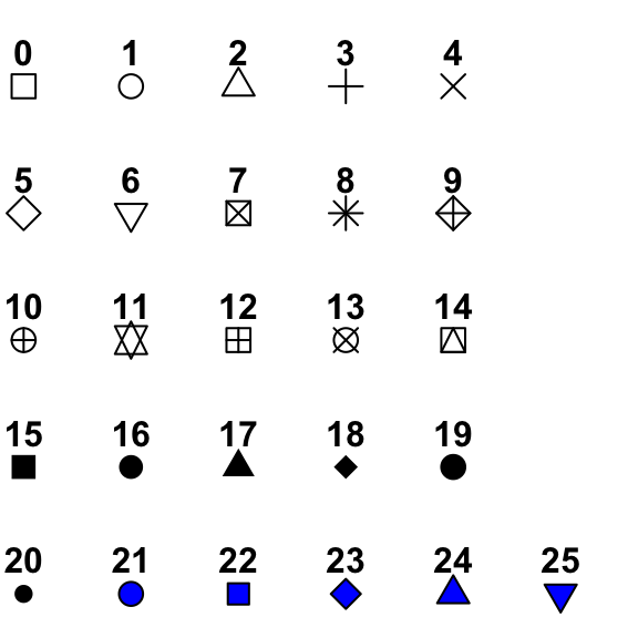
Different shapes with their codes:
Playing with variables
- in this case, the colours and size of the points is conditional on the values of the variables
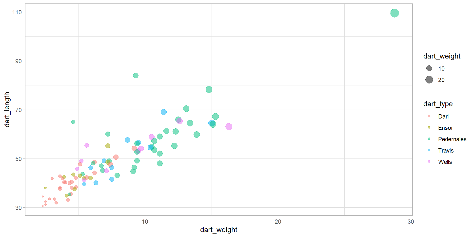
Adding text
ggplot(data = df_darts_edit)+
  aes(x = dart_weight, y = dart_length, color = dart_type, size = dart_weight)+
  geom_point(alpha = 0.5)+
  labs(
    title = "A very nice plot",
    subtitle = "Look at those colors!",
    x ="weight (g)",
    y = "length (g)",
    caption =  "Data = package Archdata",
    color = "Type of a dart",
    size = "Weight of a dart")+
  theme_classic()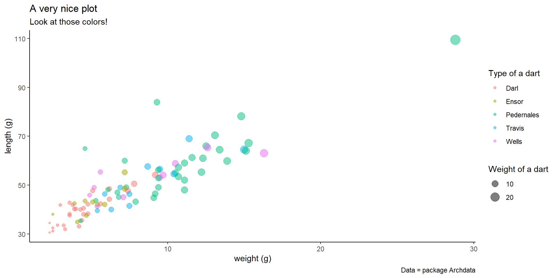
Spliting plots
ggplot(data = df_darts_edit)+
  aes(x = dart_weight, y = dart_length, color = dart_type, size = dart_weight)+
  geom_point(alpha = 0.5)+
  facet_wrap(~dart_type)+
  labs(
    title = "A very nice plot",
    subtitle = "Look at those colors!",
    x ="weight (g)",
    y = "length (g)",
    caption =  "Data = package Archdata",
    color = "Type of a dart",
    size = "Weight of a dart")+
  theme_light()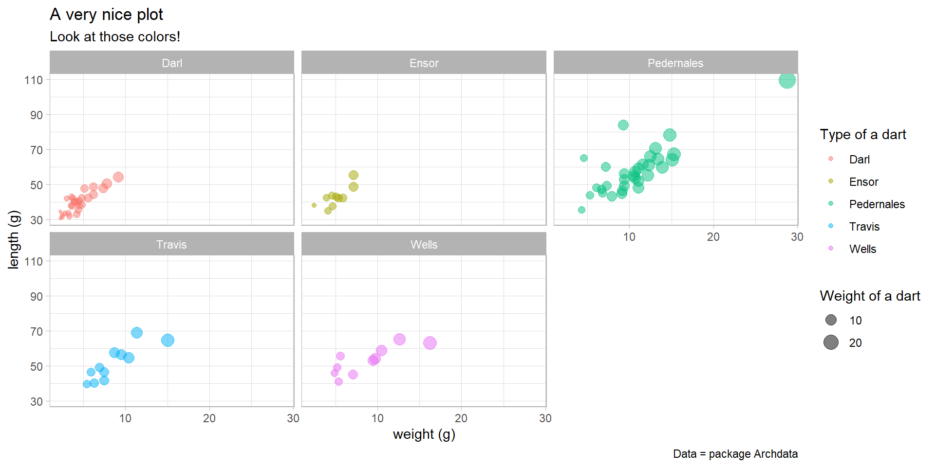
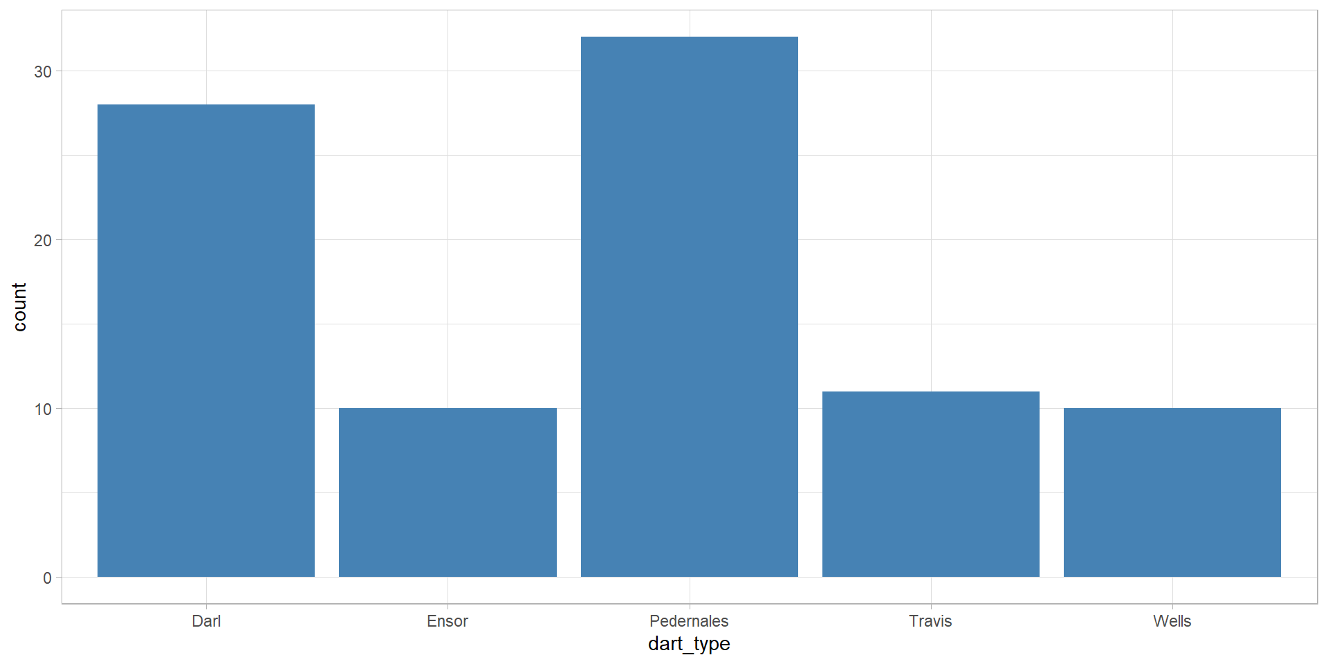
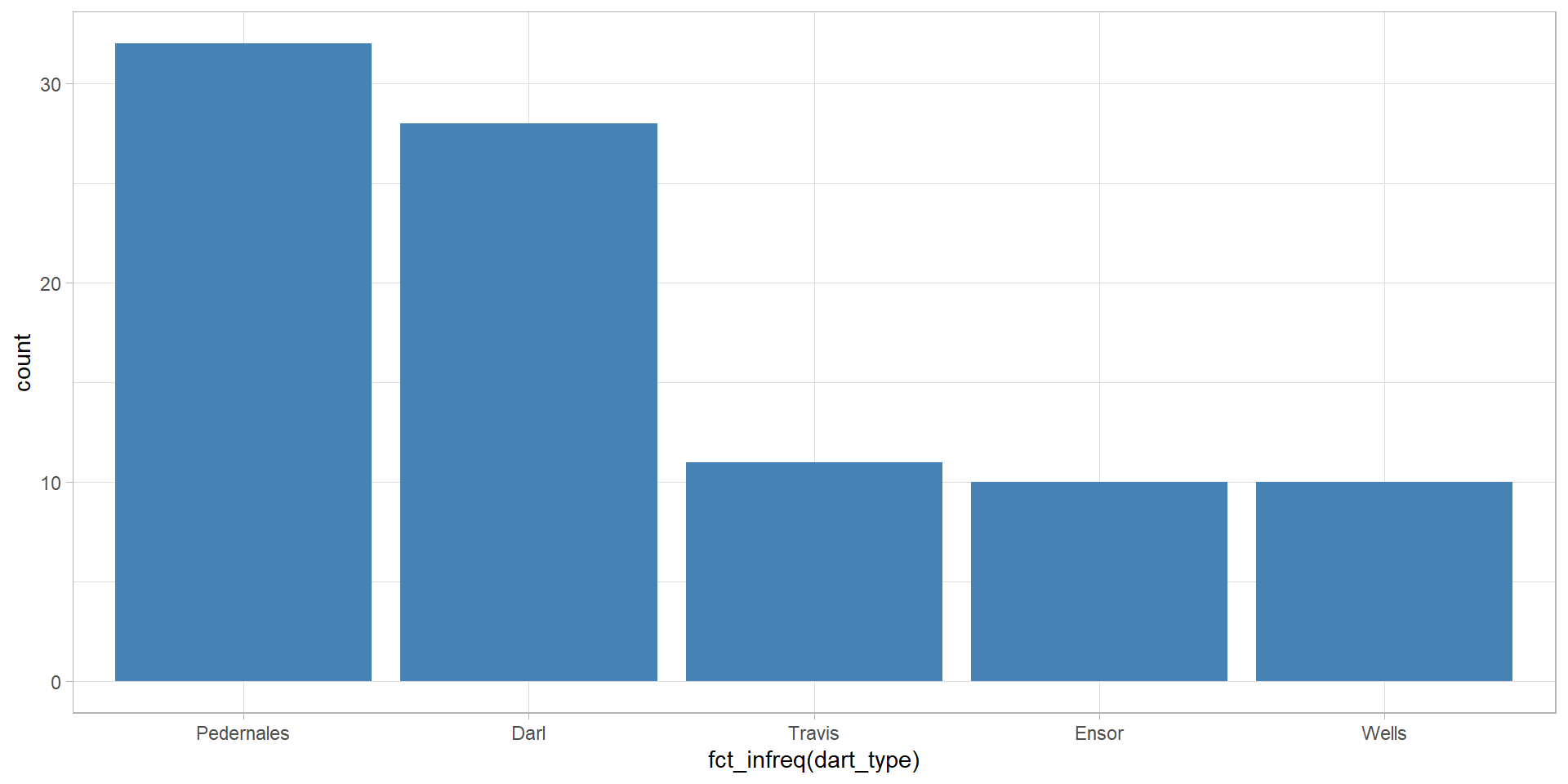
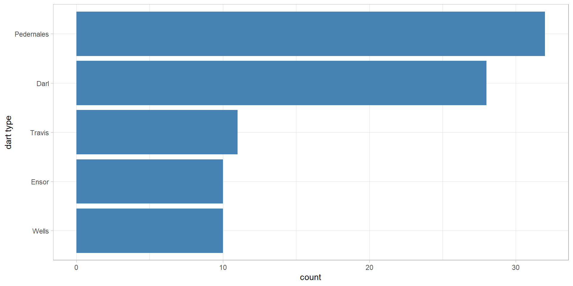
Back to barplots

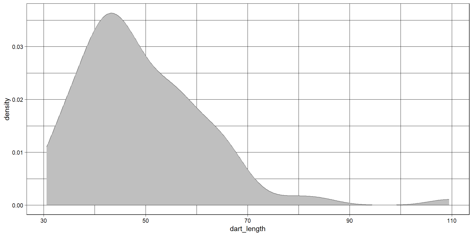
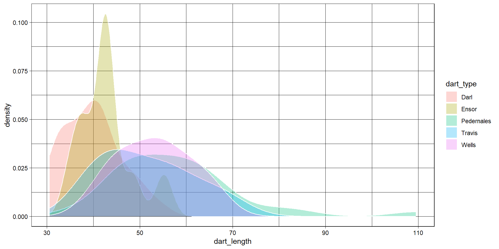
Back to the density plot
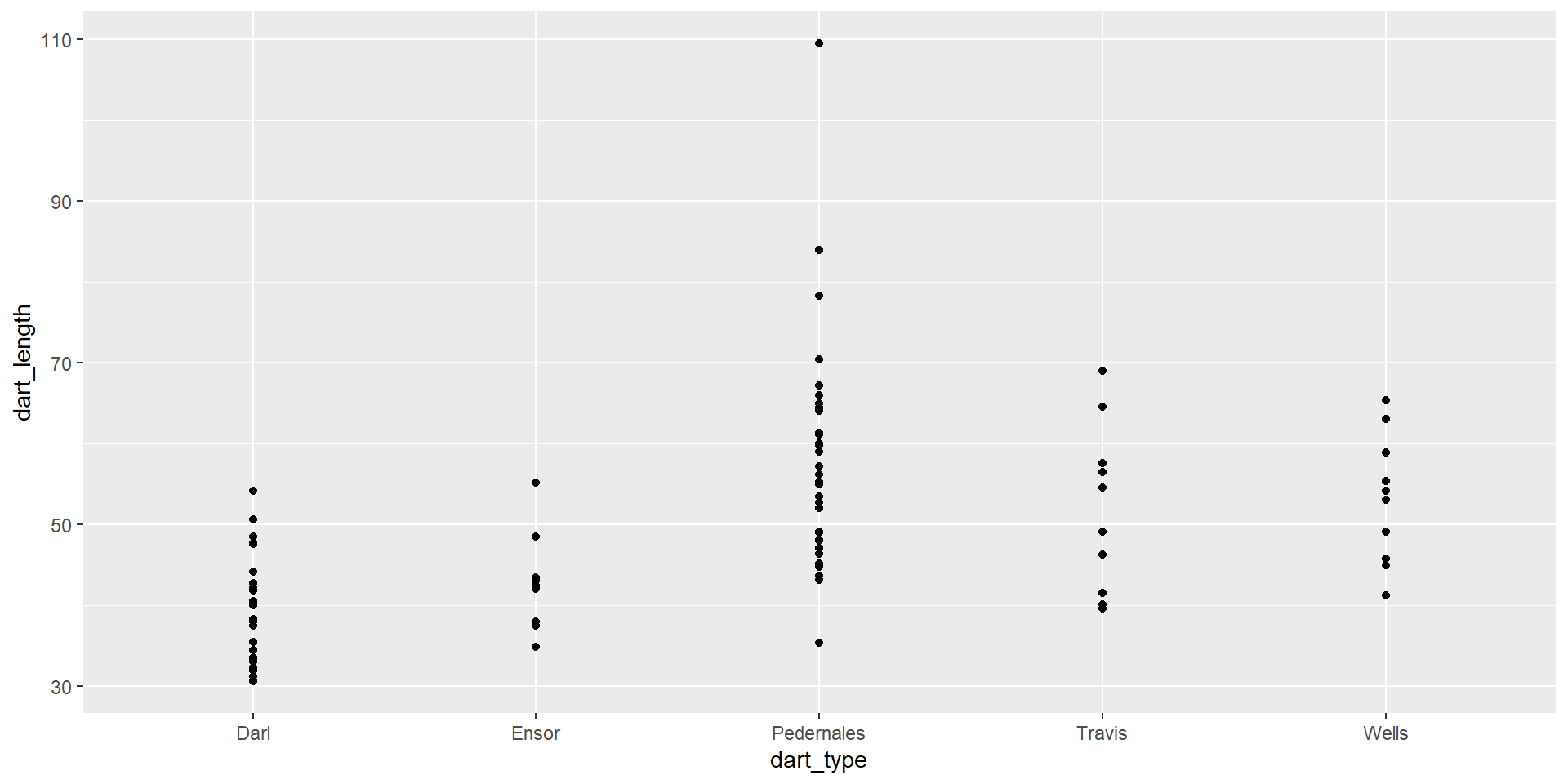
Points instead of boxplots
Solution
    RD   ND   SD   H  NH       Phase
1 11.1 10.0 10.3 5.5 2.5 Subapennine
2  9.5  9.2  9.8 4.8 2.0 Subapennine
3 20.8 20.9 22.0 9.5 3.8 Subapennine
4 19.5 18.2 19.5 8.8 2.7 Subapennine
5 15.5 15.5 18.8 9.8 3.2 Subapennine
6 11.7 11.1 11.5 3.8 1.4 Subapennine'data.frame': 60 obs. of 6 variables:
$ RD : num 11.1 9.5 20.8 19.5 15.5 11.7 10.8 15 18.5 11 ...
$ ND : num 10 9.2 20.9 18.2 15.5 11.1 10.7 16.1 16.4 8.9 ...
$ SD : num 10.3 9.8 22 19.5 18.8 11.5 10.8 16.4 18 9.5 ...
$ H : num 5.5 4.8 9.5 8.8 9.8 3.8 3.5 11.8 10.5 5.8 ...
$ NH : num 2.5 2 3.8 2.7 3.2 1.4 1.7 3.5 4.8 3.7 ...
$ Phase: chr "Subapennine" "Subapennine" "Subapennine" "Subapennine" ...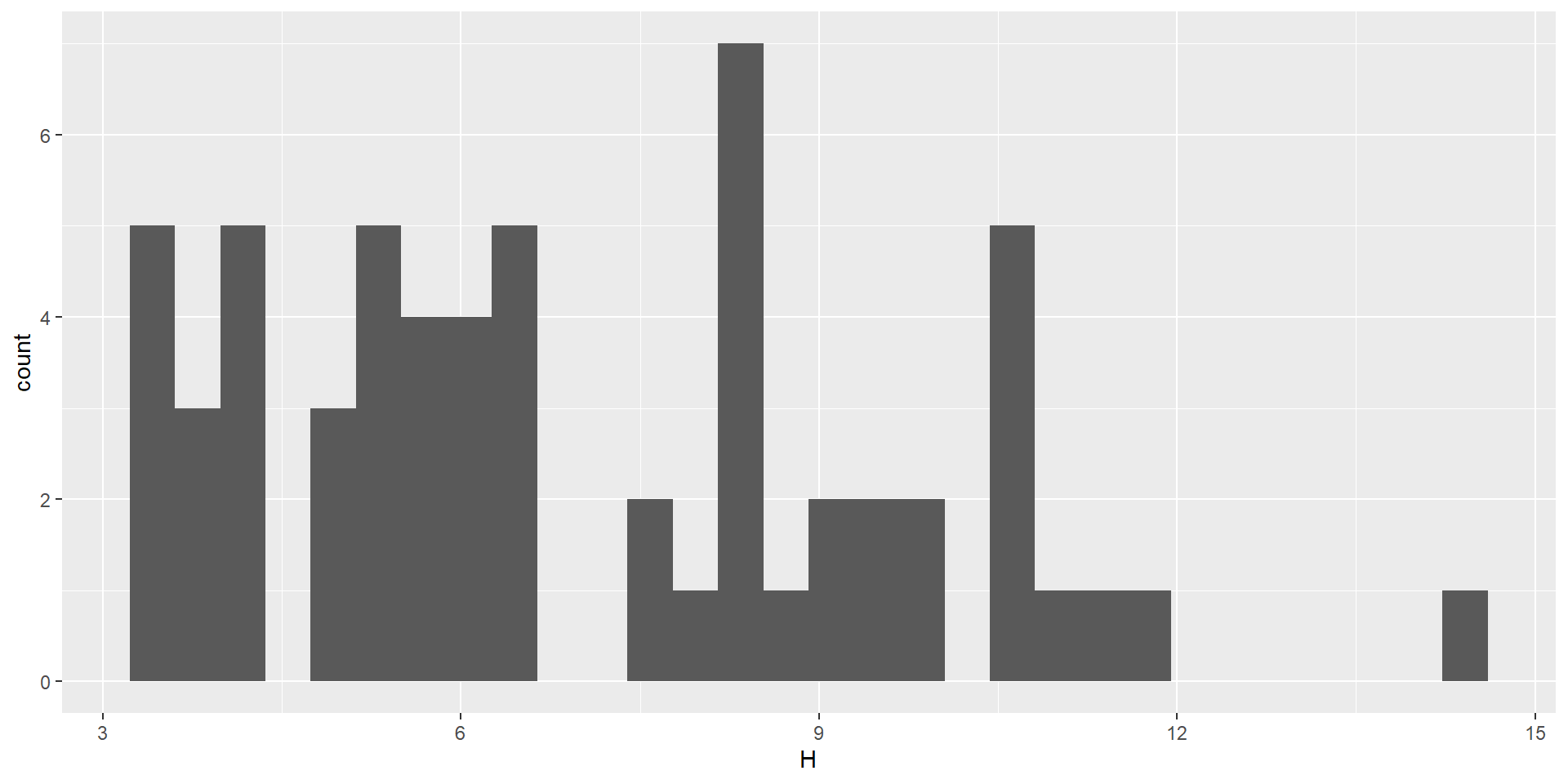
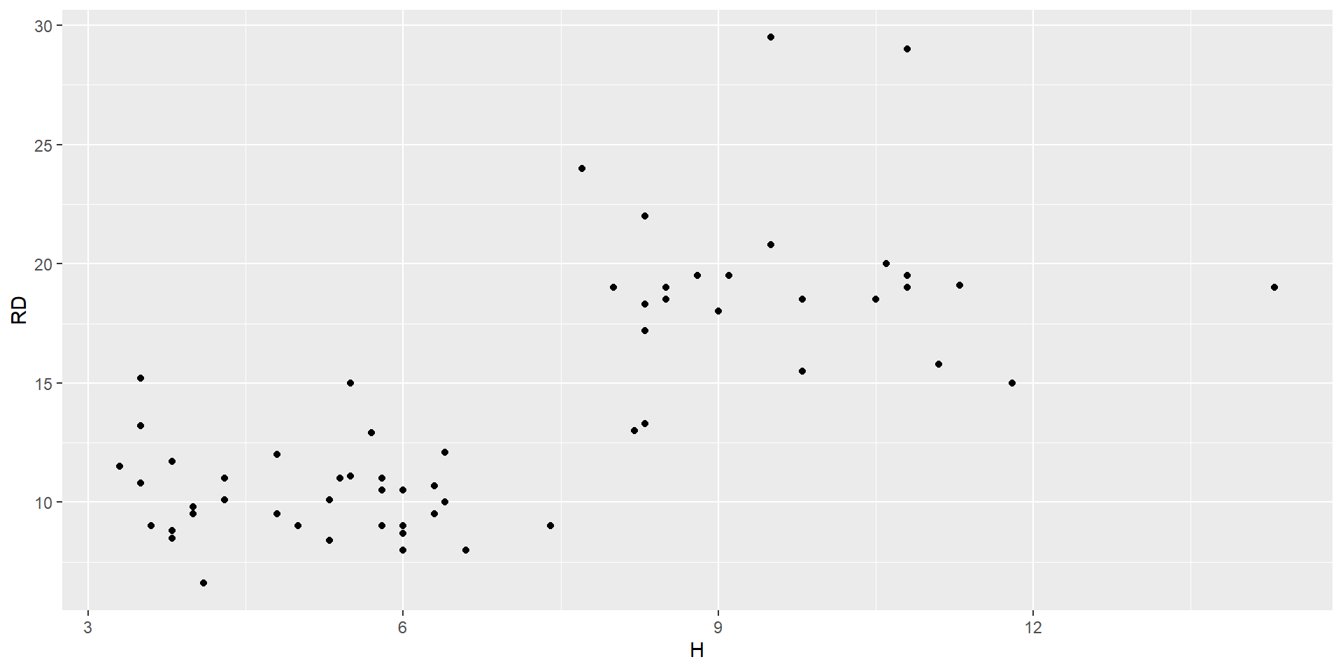
ggplot(data = df_cups)+
  aes(x = H, y = RD, color = Phase)+
  geom_point(size = 4, alpha = 0.5)+
  labs(x = "Height", y = "Rim Diameter")+
  theme_light()