Correspondence analysis

Goals

new ways of data manipulation
- combining vectors into dataframe
- columns, rows and values selection
- mathematical operations in rows
some fancy stuff to make your ggplot look better
introduction to the correspondence analysis in R

Data Manipulation

Vectors

you already know vector - a combination of several values stored in a single object

cisla <- c(1:10)
cisla

 [1]  1  2  3  4  5  6  7  8  9 10

stovky <- c(101:110)
stovky

 [1] 101 102 103 104 105 106 107 108 109 110

pismena <- c("a", "b", "c", "d", "e", "f", "g", "h", "i", "j")
pismena

 [1] "a" "b" "c" "d" "e" "f" "g" "h" "i" "j"

Combining different vectors with rbind and cbind

you can combine different vectors into matrixes or dataframes
rbind() combine vectors into Rows, cbind() into Columns
the vectors have to be of the same length!
cbind

sloupce <- cbind(cisla, stovky, pismena)
head(sloupce, 5)

     cisla stovky pismena
[1,] "1"   "101"  "a"    
[2,] "2"   "102"  "b"    
[3,] "3"   "103"  "c"    
[4,] "4"   "104"  "d"    
[5,] "5"   "105"  "e"

rbind

radky <- rbind(cisla, stovky, pismena)
radky

        [,1]  [,2]  [,3]  [,4]  [,5]  [,6]  [,7]  [,8]  [,9]  [,10]
cisla   "1"   "2"   "3"   "4"   "5"   "6"   "7"   "8"   "9"   "10" 
stovky  "101" "102" "103" "104" "105" "106" "107" "108" "109" "110"
pismena "a"   "b"   "c"   "d"   "e"   "f"   "g"   "h"   "i"   "j"

Dataframe

You can then very simply create a dataframe:

tabulka <- data.frame(sloupce)

But you have to check whether the numbers are really numbers

str(tabulka)

'data.frame':   10 obs. of  3 variables:
 $ cisla  : chr  "1" "2" "3" "4" ...
 $ stovky : chr  "101" "102" "103" "104" ...
 $ pismena: chr  "a" "b" "c" "d" ...

Whoa! The numbers are not numbers but characters. You will have to fix it by as.numeric() if you want to do mathematical operations. It is also a good practice to always check the structure of your dataframe before carrying out any operations.

tabulka$cisla <- as.numeric(tabulka$cisla)
tabulka$stovky <- as.numeric(tabulka$stovky)
str(tabulka)

'data.frame':   10 obs. of  3 variables:
 $ cisla  : num  1 2 3 4 5 6 7 8 9 10
 $ stovky : num  101 102 103 104 105 106 107 108 109 110
 $ pismena: chr  "a" "b" "c" "d" ...

Square brackets

  cisla stovky pismena
1     1    101       a
2     2    102       b
3     3    103       c
4     4    104       d

with square brackets [] you can easily select specific columns, rows or cells
your_dataframe[row number, column number]
1st row:

tabulka[1,]

  cisla stovky pismena
1     1    101       a

1st column:

tabulka[,1]

 [1]  1  2  3  4  5  6  7  8  9 10

value in the 1st row and 2nd column:

tabulka[1,2]

[1] 101

Mathematics in dataframes

Now you can make some mathematical operations by selecting specific cells with square brackets:

tabulka[1,2] + tabulka[2,2]

[1] 203

You can even create a new column with the results:

tabulka$novy_sloupec <-tabulka[,1] + 10
head(tabulka, 4)

  cisla stovky pismena novy_sloupec
1     1    101       a           11
2     2    102       b           12
3     3    103       c           13
4     4    104       d           14

or alternatilevy use mutate() function from dplyr package

library(dplyr)
tabulka<-mutate(tabulka, este_jeden_sloupec = tabulka[,1] + 100)
head(tabulka,4)

  cisla stovky pismena novy_sloupec este_jeden_sloupec
1     1    101       a           11                101
2     2    102       b           12                102
3     3    103       c           13                103
4     4    104       d           14                104

rowSums

you can calculate sums of specific columuns in each row by rowSums()

tabulka_1 <- tabulka
tabulka_1$sucet <- rowSums(tabulka_1[,1:2])
head(tabulka_1, 4)

  cisla stovky pismena novy_sloupec este_jeden_sloupec sucet
1     1    101       a           11                101   102
2     2    102       b           12                102   104
3     3    103       c           13                103   106
4     4    104       d           14                104   108

altenative solution in dplyr:

tabulka <- tabulka %>% 
  mutate(sucet = cisla + stovky)
head(tabulka,4)

  cisla stovky pismena novy_sloupec este_jeden_sloupec sucet
1     1    101       a           11                101   102
2     2    102       b           12                102   104
3     3    103       c           13                103   106
4     4    104       d           14                104   108

colnames

sometimes you will need to select names of the columns to rename them or create specific vector from them
you can manipulate with column names with function colnames()

nazvy_sloupcu <- colnames(tabulka)
nazvy_sloupcu

[1] "cisla"              "stovky"             "pismena"           
[4] "novy_sloupec"       "este_jeden_sloupec" "sucet"

Let’s have a look on table radky, the colnames look bit strange

data.frame(radky)

         X1  X2  X3  X4  X5  X6  X7  X8  X9 X10
cisla     1   2   3   4   5   6   7   8   9  10
stovky  101 102 103 104 105 106 107 108 109 110
pismena   a   b   c   d   e   f   g   h   i   j

Let’s say we will name the columns after the values in pismena row

colnames(radky)<- radky[3,]
head(radky, 4)

        a     b     c     d     e     f     g     h     i     j    
cisla   "1"   "2"   "3"   "4"   "5"   "6"   "7"   "8"   "9"   "10" 
stovky  "101" "102" "103" "104" "105" "106" "107" "108" "109" "110"
pismena "a"   "b"   "c"   "d"   "e"   "f"   "g"   "h"   "i"   "j"

You can also remove row used for column names:

radky <- radky[-3,]
radky<-data.frame(radky)
radky

         a   b   c   d   e   f   g   h   i   j
cisla    1   2   3   4   5   6   7   8   9  10
stovky 101 102 103 104 105 106 107 108 109 110

Exercise

copy, paste and run this chunk code from our website:

datace <- c("ne.lin", "ne.lin", "en.zvo", "ne.lin", "en.zvo", "en.zvo")
nadoby <- c(4, 3, 7, 2, 4, 3)
sipy <- c(0,1,3,0, 2, 4)
cu_dycka <- c(0,0,3,0, 4,2)
spondyl <- c(5,2,0,4, 0, 0)
kopytovity_klin <- c(4,5,0,4, 0, 0)
desticka <- c(0,0,2,0,1, 3)
zrnoterka <- c(1, 0, 0, 1, 0, 0)

pohrebiste <- data.frame(datace, nadoby, sipy, cu_dycka, spondyl, kopytovity_klin, desticka, zrnoterka)

pohrebiste

  datace nadoby sipy cu_dycka spondyl kopytovity_klin desticka zrnoterka
1 ne.lin      4    0        0       5               4        0         1
2 ne.lin      3    1        0       2               5        0         0
3 en.zvo      7    3        3       0               0        2         0
4 ne.lin      2    0        0       4               4        0         1
5 en.zvo      4    2        4       0               0        1         0
6 en.zvo      3    4        2       0               0        3         0

create a new column with the sum of the artefacts found in each grave
create a new column called “ID” where each grave has an unique number

Solution

create a new column with the sum of the artefacts found in each grave

pohrebiste_2 <- pohrebiste
pohrebiste_2$pocet_artefaktu <- rowSums(pohrebiste[, 2:8])
pohrebiste_2$ID <- c(1:6)
pohrebiste_2

  datace nadoby sipy cu_dycka spondyl kopytovity_klin desticka zrnoterka
1 ne.lin      4    0        0       5               4        0         1
2 ne.lin      3    1        0       2               5        0         0
3 en.zvo      7    3        3       0               0        2         0
4 ne.lin      2    0        0       4               4        0         1
5 en.zvo      4    2        4       0               0        1         0
6 en.zvo      3    4        2       0               0        3         0
  pocet_artefaktu ID
1              14  1
2              11  2
3              15  3
4              11  4
5              11  5
6              12  6

alternative solution with package dplyr:

pohrebiste <- pohrebiste %>% 
  mutate(pocet_artefaktu= rowSums(pohrebiste[,2:8]),
         ID = c(1:6))

head(pohrebiste, 3)

  datace nadoby sipy cu_dycka spondyl kopytovity_klin desticka zrnoterka
1 ne.lin      4    0        0       5               4        0         1
2 ne.lin      3    1        0       2               5        0         0
3 en.zvo      7    3        3       0               0        2         0
  pocet_artefaktu ID
1              14  1
2              11  2
3              15  3

Correspondence analysis (CA)

A bit of theory

one of the multivatiate statistical methods
suitable for contingency tables (kontingenční tabulka) where you have counts of two or more categorical variables
one type of variable are stored in rows, other in columns
typicaly, you can visualise result of CA with scatterplots

A simple contingency table

now, have a look at this simple contingency table of an fictional Bell Beaker burial site: one variable is sex of buried individuals (columns), second the position of their bodies (rows)

	male	female
left side	10	1
right side	2	12

already from the first sight it is obvious that females were predominantly buried on their right site and male on their left site
correspondence analysis will help you when your contingency table have much more variables and the relations between variables are then much harder to observe

Use of CA

typical archaeological uses of CA:
- seriation
- counts of different types of artefacts (eg. artefacts in burial sites, types of chipped stone industry,…)
- presence or absence of different features in archaeological collections (e.g.presence or absence of construction elements in graves)
it works only with discrete numbers (celá čísla) - i.e. counts, or dichotomies (presence / absence, 1/0)

Quick correspondence analysis

imagine we have a burial site and want to observe relation between numbers of different types of artefacts found in the graves and between datations of the graves

Research questions

are there certain types of artefacts related to certain datations?
are there differencies within the different datations?

Materials and methods

we will use the fictional data from the last exercise, the dataframe “pohrebiste”
TASKS:
- clean your workplace and load the “pohrebiste” data from our webpage again
- install and load package ca

  datace nadoby sipy cu_dycka spondyl kopytovity_klin desticka zrnoterka
1 ne.lin      4    0        0       5               4        0         1
2 ne.lin      3    1        0       2               5        0         0
3 en.zvo      7    3        3       0               0        2         0
4 ne.lin      2    0        0       4               4        0         1
5 en.zvo      4    2        4       0               0        1         0
6 en.zvo      3    4        2       0               0        3         0

Results

library(ca)
ca_vysledek <- ca(pohrebiste[,2:8])
plot(ca_vysledek)

notice we are running the analysis only with columns which represent number of artefacts (2nd to 8th)
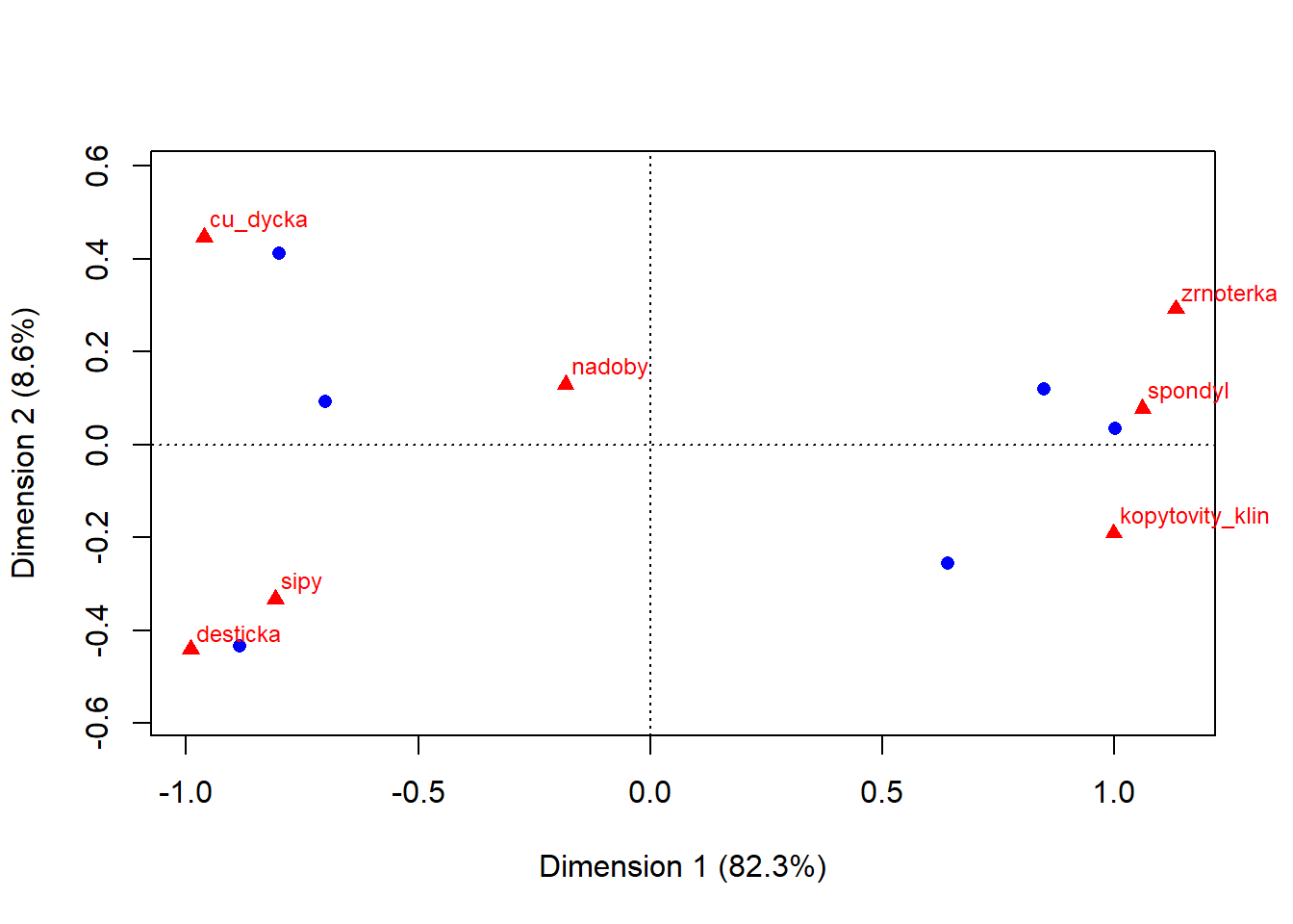
also notice there are two types of points in the plot:
- blue circles represent row values, which are in this case graves
- red triangles represent column values - numbers of specific artefacts

Interpretation

there are two clearly distinct groups of graves with distinct types of artefacts
on the other hand number of vessels seems to be indifferent to the groups - both grave groups share similar number of ceramic vessels
the x axis explains 82 % of the difference between graves and artefacts, y axis only 9 %. This mean that the difference between those two groups is bigger then within them. In other words, the difference between e.g. copper dagger (cu_dycka) and spondylus is much much greater then between the copper dagger and arrow heads (sipy)

Now let’s have a closer look

ca_vysledek


 Principal inertias (eigenvalues):
           1        2        3        4        5       
Value      0.667126 0.069873 0.054181 0.018769 0.001128
Percentage 82.25%   8.61%    6.68%    2.31%    0.14%   


 Rows:
            [,1]      [,2]      [,3]     [,4]      [,5]      [,6]
Mass    0.189189  0.148649  0.202703 0.148649  0.148649  0.162162
ChiDist 0.879868  0.836034  0.738122 1.026842  0.926948  1.011206
Inertia 0.146464  0.103898  0.110437 0.156736  0.127724  0.165817
Dim. 1  1.037358  0.783658 -0.856640 1.225783 -0.979198 -1.083841
Dim. 2  0.450424 -0.963242  0.350276 0.134612  1.561622 -1.635249


 Columns:
           nadoby      sipy  cu_dycka  spondyl kopytovity_klin  desticka
Mass     0.310811  0.135135  0.121622 0.148649        0.175676  0.081081
ChiDist  0.300899  0.875803  1.086977 1.097286        1.064182  1.129904
Inertia  0.028141  0.103653  0.143698 0.178978        0.198950  0.103515
Dim. 1  -0.224254 -0.989256 -1.177308 1.297475        1.221578 -1.212896
Dim. 2   0.489148 -1.259831  1.692644 0.297174       -0.720551 -1.666812
        zrnoterka
Mass     0.027027
ChiDist  1.415361
Inertia  0.054142
Dim. 1   1.385408
Dim. 2   1.106622

you can see that this is not a dataframe, but a so called “list” with much complicated structure. Even so, it is possible to extract coordinates of the points (we will show it later) and use them for other analysis or visualisation in ggplot.

The structure of the CA result

this looks even more complicated, but don’t worry!

str(ca_vysledek)

List of 16
 $ sv        : num [1:5] 0.8168 0.2643 0.2328 0.137 0.0336
 $ nd        : logi NA
 $ rownames  : NULL
 $ rowmass   : num [1:6] 0.189 0.149 0.203 0.149 0.149 ...
 $ rowdist   : num [1:6] 0.88 0.836 0.738 1.027 0.927 ...
 $ rowinertia: num [1:6] 0.146 0.104 0.11 0.157 0.128 ...
 $ rowcoord  : num [1:6, 1:5] 1.037 0.784 -0.857 1.226 -0.979 ...
  ..- attr(*, "dimnames")=List of 2
  .. ..$ : NULL
  .. ..$ : chr [1:5] "Dim1" "Dim2" "Dim3" "Dim4" ...
 $ rowsup    : logi(0) 
 $ colnames  : chr [1:7] "nadoby" "sipy" "cu_dycka" "spondyl" ...
 $ colmass   : num [1:7] 0.311 0.135 0.122 0.149 0.176 ...
 $ coldist   : num [1:7] 0.301 0.876 1.087 1.097 1.064 ...
 $ colinertia: num [1:7] 0.0281 0.1037 0.1437 0.179 0.1989 ...
 $ colcoord  : num [1:7, 1:5] -0.224 -0.989 -1.177 1.297 1.222 ...
  ..- attr(*, "dimnames")=List of 2
  .. ..$ : chr [1:7] "nadoby" "sipy" "cu_dycka" "spondyl" ...
  .. ..$ : chr [1:5] "Dim1" "Dim2" "Dim3" "Dim4" ...
 $ colsup    : logi(0) 
 $ N         : num [1:6, 1:7] 4 3 7 2 4 3 0 1 3 0 ...
 $ call      : language ca.matrix(obj = as.matrix(obj))
 - attr(*, "class")= chr "ca"

Visualising CA in ggplot

in order to visualize data in ggplot, they have to be in dataframe format
so the first step will be extracting coordinates from the CA result
in this case we will extract them from first two dimensions only

x1 <- ca_vysledek$rowcoord[,1]
x2 <- ca_vysledek$rowcoord[,2]
y1 <- ca_vysledek$colcoord[,1]
y2 <- ca_vysledek$colcoord[,2]

x1 and x2 represent coordinates of row values (graves), y1 and y2 represent column values (artefacts)
quick check:

plot(x1,x2)

Creating dataframes

now we need to create dataframes with for both row values and column values
row values (graves):
- in this step, we can combine various variables describing your objects with row values. We have added “id” and “datace”

datace <- data.frame(pohrebiste$datace)
id <- data.frame(pohrebiste$ID)
coord_datace <- data.frame(cbind(datace, x1,x2, id))
colnames(coord_datace) <- c("Datace", "X1", "X2", "ID")
head(coord_datace, 4)

  Datace         X1         X2 ID
1 ne.lin  1.0373584  0.4504244  1
2 ne.lin  0.7836584 -0.9632417  2
3 en.zvo -0.8566397  0.3502757  3
4 ne.lin  1.2257826  0.1346118  4

column values (artefacts):

artefakty <- data.frame(colnames(pohrebiste[,2:8]))
coord_artefakty <- data.frame(cbind(y1, y2))
coord_artefakty$artefakty <- rownames(coord_artefakty)
colnames(coord_artefakty) <- c("Y1", "Y2","Artefakty")
rownames(coord_artefakty) <- c(1:7)
head(coord_artefakty, 4)

          Y1         Y2 Artefakty
1 -0.2242544  0.4891476    nadoby
2 -0.9892557 -1.2598313      sipy
3 -1.1773081  1.6926442  cu_dycka
4  1.2974752  0.2971739   spondyl

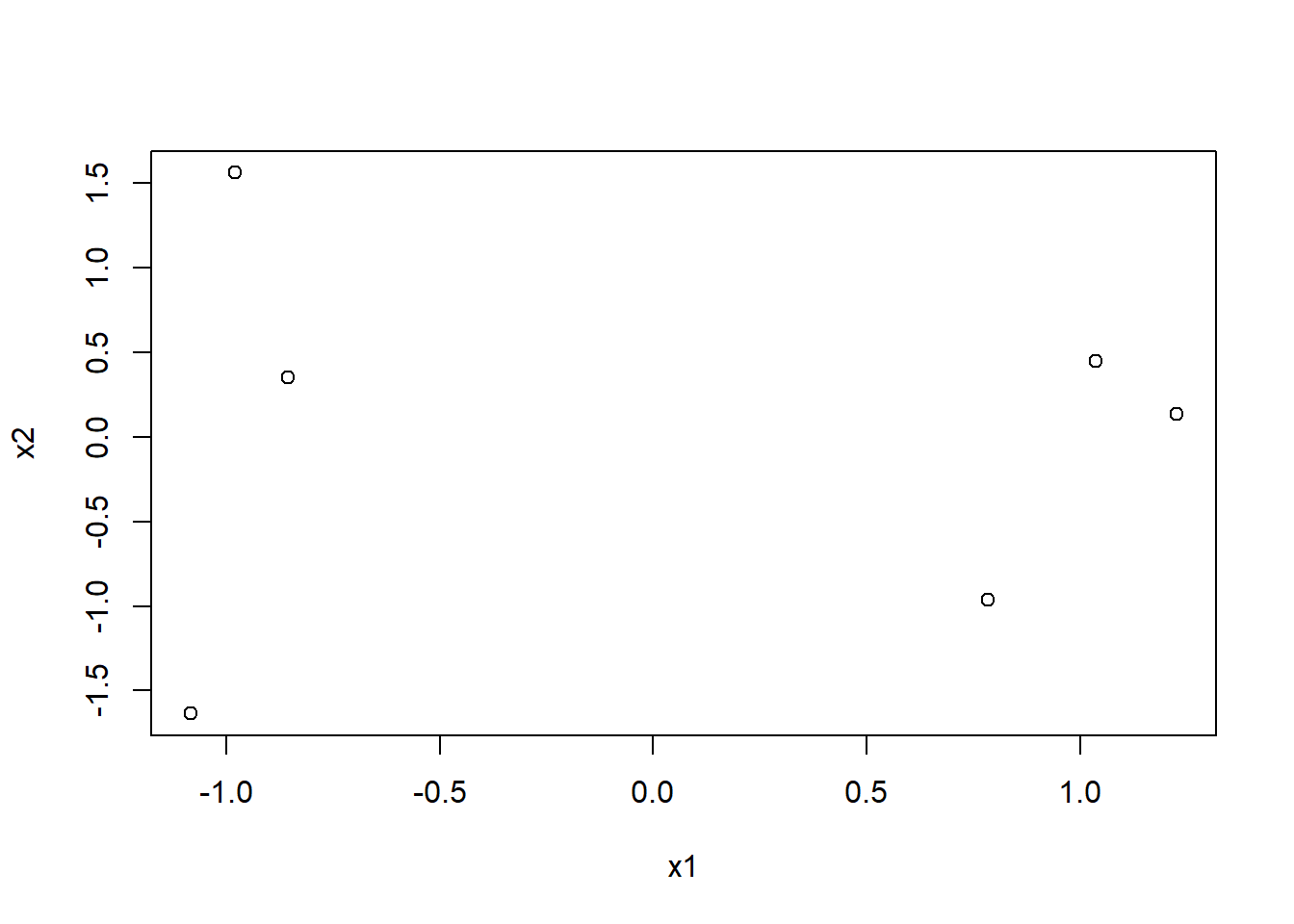
A very simple ggplot

lets have a quick ggplot

ggplot()+
  geom_point(data = coord_datace, aes(X1, X2, color = Datace))+
  geom_point(data = coord_artefakty, aes(Y1, Y2), shape = 17)

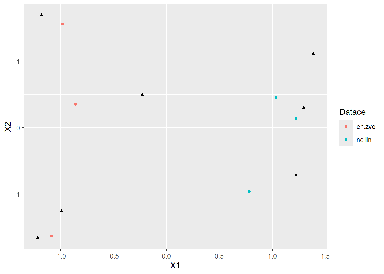
notice there are 2 types of values in 2 dataframes, so you need to call geom_point() two times
in ggplot we can also easily distinguish different datations by color

Advanced ggplot

now you can play more with adjusting the plot

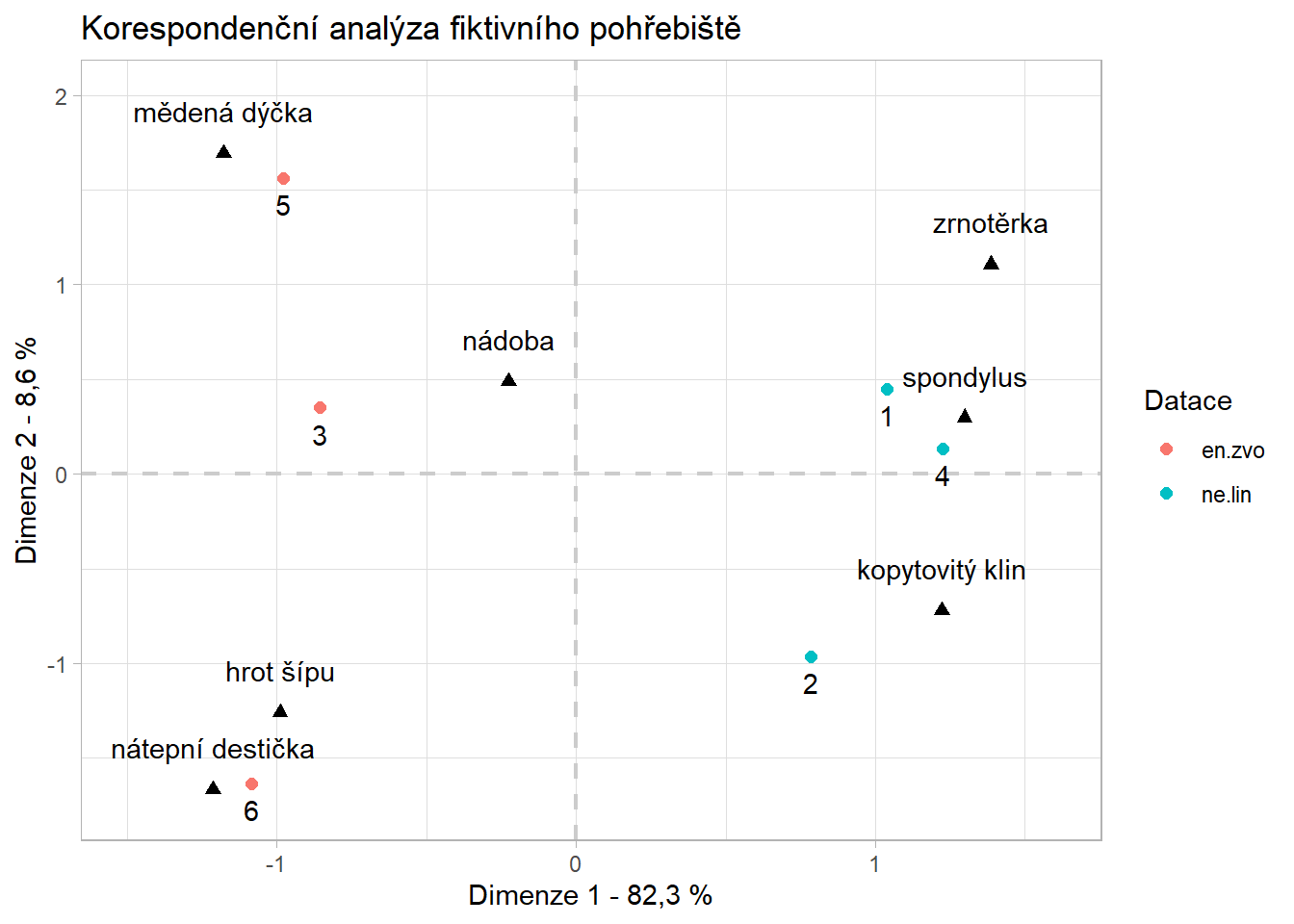
Solution

you can add text to your ggplot by geom_text()
you can also rename plot labels without the need to rename variables in your original dataframe. To do so, create a vector with label names and then specify it in geom_text(...,aes(label=your_vector))
for more tips how to adjust text see ggplot2.tidyverse.org

labels_artefacts <- c("nádoba", "hrot šípu", "mědená dýčka", "spondylus", "kopytovitý klin", "nátepní destička", "zrnotěrka")

ggplot()+
  geom_vline(xintercept = 0, color="gray80", linewidth = 0.75, linetype = "dashed")+
  geom_hline(yintercept = 0, color="gray80", linewidth = 0.75, linetype = "dashed")+
  geom_point(data = coord_datace, aes(X1, X2, colour = Datace), size = 2)+
  geom_point(data = coord_artefakty, aes(Y1, Y2), shape = 17, size = 2)+
  geom_text(data = coord_artefakty, aes(label = labels_artefacts, x=Y1, y=Y2), vjust = -1.5)+
  geom_text(data = coord_datace, aes(label = ID, x=X1, y=X2), vjust = 1.75)+
  xlim(-1.5, 1.6)+
  ylim(-1.75, 2)+
  labs(x="Dimenze 1 - 82,3 %", y="Dimenze 2 - 8,6 %",
       title = "Korespondenční analýza fiktivního pohřebiště")+
  theme_light()